Transcription
Hierarchical ModelsDavid M. BleiOctober 17, 20111Introduction We have gone into detail about how to compute posterior distributions. Now we are going to start to talk about modeling tools—the kinds of components thatcan be used in data models on which we might want to compute a posterior. Notice that we can talk about models independently of inference. In this segment of the class, we’ll introduce and review the other basic building blocksof models– Mixture models– Mixed membership models– Regression models– Matrix factorization models– Models based on time and space2What is a hierarchical model? There isn’t a single authorative definition of a hierarchical model. Gelman et al., 2004– “Estimating the population distribution of unonobserved parameters”– “Multiple parameters related by the structure of the problem”1
Knowing something about one “experiment” tells us something about another.– Multiple similar experiments– Similar measurements from different locations– Several tasks to perform on the same set of images “Sharing statistical strength.” The idea here is that something we can infer well in onegroup of data can help us with something we cannot infer well in another. For example,we may have a lot of data from California but much less data from Oregon. What welearn from California should help us learn in Oregon. Key idea: Inference about one unobserved quantity affects inference about anotherunobserved quantity.– Includes some traditional hierarchical models– Does not include calling a prior/likelihood a hierarchical model– Includes models not necessarily thought of as hierarchical, such as HMMs, Kalmanfilters, mixtures of Gaussians.– (As such, it might be too forgiving a “definition.”)3The classical hierarchical model The classical hierarchical model looks like this:Fixed hyperparameterShared hyperparameterPer-group parametersMultiple groups of observations We observe multiple groups of observations, each from its own parameter. The distribution of the parameters is shared by all the groups. It too has a distribution.2
Inference about one group’s parameter affects inference about another group’s parameter.– You can see this from the Bayes ball algorithm.– Look back at the properties of hierarchical models. See how they apply here.– Consider if the shared hyperparameter were fixed. This is not a hierarchicalmodel. Intuitive example: Height measurements of 8 year old daughters from different families.– Which family you are in will affect your height.– Assume each measurement is from a Gamma with an unknown per-family mean.– When we observe 1000 kids in a family, what do we know about the mean?– How about when we observe 10 kids in a family? How about 1?– What do we know about a new family that we haven’t met? Let’s show mathematically how information is transmitted in the predictive distribution. A more concrete (but still abstract) model– Assume m groups and each group has n i observations.– Assume fixed hyperparameters α. Consider the following generative process—– Draw θ F0 (α).– For each group i {1, . . . , m}:* Draw µ i θ F1 (θ ).* For each data point j {1, . . . , n j }:· Draw x i j µ i F2 (µ j ). To make this more concrete, consider all distributions to be Gaussian, and the data tobe real valued. Or, set F0 , F1 and F1 , F2 to be a chain of conjugate pairs of distributions. Let’s consider the posterior distribution of the i th groups parameter given the data(including the data in the i th group).3
– Notice: we are not yet worrying about computation. We can still investigateproperties of the model conditioned on data. The posterior distribution isp (µ i D ) ZÃp(θ α) p(µ i θ ) p(x i µ i )YZ!p(µ j θ ) p(x j µ j ) d µ j d θ(1)j 6 i Inside the integral, the first and third term together are p(x i , θ α). This can beexpressed asp(x i , θ α) p(x i α) p(θ x i ), α).(2)Note that p(x i α) does not depend on θ or µ i . This reveals that the per-group posterior isZp(µ i D ) p(θ x i , α) p(µ i θ ) p(x i µ i ) d θ(3) In other words, the other data influence our inference about the parameter for group ithrough their effect on the distribution of the hyperparameter. When the hyperparameter is fixed, the other groups do not influence our inferenceabout the parameter for group i . Notice that in contemplating this posterior, the group in question does not influence itsidea of the hyperparameter. Let’s turn to how the other data influence θ . From our knowledge of graphical models,we know that it is through their parameters µ j . However, we can also see it directly byunpacking the posterior p(θ x i ). The posterior of the hyperparameter θ given all but the i th group isYZp(θ x i , α) p(θ α)p(µ j θ ) p(x j µ j ) d µ j(4)j 6 i (This gets fuzzy here.) Construe each integral as a weighted average of p(µ j θ ) weightedby p(x j µ j ) for each value of µ j .4
Suppose this is dominated by one of the values, call it µ̂ j . Then we can see the posterior asp(θ x i , α) p(θ α)Yp(µ̂ j θ )(5)j 6 i This looks a lot like a prior/likelihood set-up. E.g., if p(θ α) and p(µ̂ j θ ) form aconjugate pair then this is a conjugate posterior distribution of θ . It suggests that the hyperparameter is influened by the groups of data through whateach one says about its respective parameter. This is not “real” inference, but it illustrates how information is transmitted.– Other groups tell us something about their parameters.– Those parameters tell us something about the hyperparameter.– The hyperparameter tells us something about the group in question. In Normal-Normal models, exact inference is possible.– However, in general p(α D ) does not have a nice form.– Notice that the GM is always a tree.– The problem is the functional form of the relationships between nodes. You can imagine how the variational inference algorithm transmits information backand forth. (Gibbs sampling and methods for exact inference do the same.) Consider other computations, conditioned on data.– The predictive distribution for a known group p( xnew D ) will depend on otherigroups (for the hyperparameter) and on other data within the same group (for theper-group parameter).– The distribution of a parameter for a totally unobserved group µnew will dependon the posterior of hyperparameter θ conditioned on all the data.4Hierarchical regression One of the main application areas of hierarchical modeling is to regression.5
Hierarchical (or multilevel) modeling allows us to use regression on complex data sets.– Grouped regression problems (i.e., nested structures)– Overlapping grouped problems (i.e., non-nested structures)– Problems with per-group coefficients– Random effects models (more on that later) Example: Collaborative filtering– Echonest.net has massive music data, attributes about millions of songs.– Imagine taking a data set of a user’s likes and dislikes– Can you predict what other songs he/she will like or dislike?– This is the general problem of collaborative filtering.– Note: We also have information about each artist.– Note: There are millions of users. Example: Social data– We measured the literacy rate at a number of schools.– Each school has (possibly) relevant attributes.– What affects literacy? Which programs are effective?– Note: Schools are divided into states. Each state has its own educational systemwith state-wide policies.– Note: Schools can be divided by their educational philosophy These kinds of problems—predictive and descriptive—can be addressed with regression. The causal questions in the descriptive analysis are difficult to answer definitively.However, we can (with caveats) still interpret regression parameters. (That said, wewon’t talk about causation in this class. It’s a can of worms.)4.1Review Bayesian regression:6
Fixed hyperparameterParameterResponsePer-data predictors Regression is a field. There are sequences of classes taught about it. Notation and terminology– Response variable yi is what we try to predict.– Predictor vector x i are attributes of the i th data point.– Coefficients β are regression parameters. The two regression models everyone has heard of are– Linear regression for continuous responses,yi x i N (β x i , σ2 )(6)– Logistic regression for binary responses (e.g., spam classification),p( yi 1 x i ) logit(β x i )(7)– In both cases, the distribution of the response is governed by the linear combination of coefficients (top level) and predictors (specific for the i th data point). We can use regression for prediction.– The coefficient component β i tells us how the expected value of the responsechanges as a function of each attribute.– For example, how does the literacy rate change as a function of the dollars spenton library books? Or, as a function of the teacher/student ratio?– How does the probability of my liking a song change based on its tempo? We can also use regression for description.7
– Given a new song, what is the expected probability that I will like it?– Given a new school, what is the expected literacy rate? Linear and logistic regression are examples of generalized linear models.– The response yi is drawn from an exponential family,p( yi x i ) exp{η(β, x i ) t( yi ) a(η(β, x i ))}.(8)– The natural parameter is a function η(β, x i ) f (β x i ).– In many cases, η(β, x i ) β x i . Discussion– In linear regression y is Gaussian; in logistic regression y is Bernoulli.– GLMs can accommodate discrete/continuous, univariate/multivariate responses.– GLMs can accommodate arbitrary attributes.– (Recall the discussion of sparsity and GLMs in COS513.) Nelder and McCallaugh is an excellent reference about GLMs. (Nelder invented them.)4.2Hierarchical regression with nested data The simplest hierarchical regression model simply applies the classical hierarchicalmodel of grouped data to regression coefficients. Nested regression:Shared but fixed hyperparameterShared hyperparameterPer-group parametersResponsePer-data predictors8
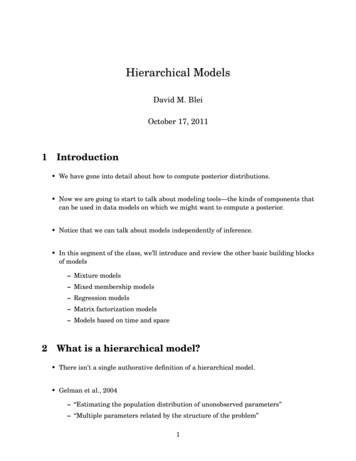
Here each group (i.e., school or user) has its own coefficients, drawn from a hyperparameter that describes general trends in the coefficients. This allows for variance at the coefficient level.– Note that the variance too is interpretable.– An attribute can make a difference in different ways for different groups (high).– An attribute can be universal in how it predicts the response (low). But since β is multivariate we have some flexibility about which components to modelhierarchically and which components to model in a fixed way for all the groups. One distinction we make in regression is between the “slope” term and “intercept” term.The intercept term is (effectively) for a coefficient that is always equal to one. Gelman and Hill (2006) draw the following useful picture:228MULTILEVEL STRUCTURESVarying interceptsVarying slopesVarying intercepts and slopesgroup Bgroup Cgroup Egroup Cgroup Egroup Eygroup Bgroup Cyygroup Agroup Dgroup Agroup Bgroup Agroup Dgroup Dx ThisxxFigure 11.1 Linear regression models with varying intercepts (y αj βx), varying slopes(y α βj x), and both (y αj βj x). The varying intercepts correspond to groupindicators astoregressionpredictors,and tercept,slope,or slopesboth representcoefficientshierarchically.x and the group indicators. The same choiceseach cofficientor subsetof coefficients.Oftenthe problemdad applymom forinformalcitycityenforcementbenefitcity indicatorsage youraceIDnameintensitylevelcoefficients.123 (Hierarchi···20will dictateIDwherewantsupportgroup-levelcoefficientsor top-level1 means19hispOaklandcal regressionhaving 1to make1 morechoices!) 0.52 1.01 1 0 0 · · · 0 .01100. 2.Also, the grouplevelwhiteparameterscanthe noise term,σ . Thus2481913 beBaltimore0.05 i.e.,1.1000 you126blackBaltimore0.051.10001errors that249arecorrelatedby 1.group. 3(ThanksMatt S. forpointingthisout.).136621black120Norfolk 0.111.08000136728hisp020Norfolk 0.111.08000 More complicated nested Figure 11.2 Some of the data from the child support study, structured as a single matrixwith one row for each person. These indicators would be used in classical regression toallow for variation among cities. In a multilevel model they are not necessary, as we codecities using their index variable (“city ID”) instead.We prefer separating the data into individual-level and city-level datasets, as in Figure11.3.9Studying the effectiveness of child support enforcement00.model00.11
Shared but fixed hyperparameterShared hyperparameterPer-group parametersShared parameterResponsePer-data predictors Back to the literacy example—– Responses are grouped by state.– Each state might have a different base literacy rate (intercept).– It increases or decreases in the same way as other schools, based on the attributes.– Or, the relationship between some attributes and literacy rates is the same for allstates; for others it varies across state. Back to the collaborative filtering example—– Responses are grouped by artist.– Each artist has a different base probability that the user will like them.– It changes in the same way as other artists, based on attributes of the song.– Or, the relationship between some attributes and probability is common for allartists; for other attributes it varies by artists. Recall the results from the previous section, and how they apply to regression.– What I know about one school tells me about others.– What I know about one artist tells me about others.– I can make a prediction about a new artist, even if they have new coefficients.– I can make a prediction about a new school, before observing data from it. A note on computation10
– As above, Normal priors and linear regression gives itself to exact inference.– However, other response variables (e.g., binary) and other priors do not.– The normal prior can be limiting, especially if you want to use tools like Laplacepriors or spike and slab priors to find sparse solutions. (Recall COS513.)4.3Nested data with per-group covariates Hierarchical regression immediately lets us reason about groups. In classical regression, per-group (e.g., state) attributes are encoded within the data.For example, how many dollars does this state apply to literacy programs? Encoding them in the groups themselves is more natural. The most complicated nested regression I can think of:Shared hyperparameterPer-group predictorsPer-group parametersShared parameterResponsePer-data predictorsThe shared parameter involves the per-group predictors (and possibly the per-datapredictors). The per-group parameters involves some or all of the per-data predictors. Also consider artists in the collaborative filtering example.– We might have descriptions of each artist (in fact, we do).– We can form a term vector and predict the “baseline” of whether the user will likea song by that artist. This helps predictions on new songs by new artists.11
4.4Regression with non-nested data So far, we considered grouped or nested data. Hierarchical modeling can capture more complicated relationships between the hiddenvariables. Thus, it can capture more complicated relationships between the observations. Suppose each data point is associated with multiple groups.– The per-data coefficients are a sum of their group coefficients.– Suppose there are G possible groups.– Let g i be the per-data group memberships, a G binary vector. These membershipsare given, along with the per-data predictors x i .– In this model,β g F0 (α)yi for g {1, . . . ,G } F1 (( g i β) x i )(9)(10) Graphical models are less useful here—the structure of how the data relate to eachother is encoded in g i .Shared hyperparameterPer-group parametersShared parameterResponsePer-data groupmembershipsPer-data predictors Here we don’t need the per-group parameters to come from a random hyperparameter.They exhibit sharing automatically because data are members of multiple groups. And it can get more complicated still:12
– Local parameters in a time series– Coefficients that aren’t observed (i.e., random effects)– Parameters in a tree– Hierarchies in hierarchies For example, a mammoth model of the Echonest dataUser predictorsUser parametersUser/artist parametersShared parameterShared artist parametersArtist predictorsRatingSong predictorsSong parametersShared song parameters– Multiple users allow many kinds of parameters and predictors– Songs are within artists; users rate all songs– Some songs might be universally popular– Some artists might be popular within users– Anything is possible– Searching within models is difficult. But first, let’s get back to a simple hierarchical model from the 1950s.5Empirical Bayes and James-Stein estimation An empirical Bayes estimate is a data-based point estimate of a hyperparameter.13
Gelman et al. point out that this is an approximation to a hierarchical model, i.e., whenwe have a posterior distribution of a hyperparameter. But empirical Bayes has an interesting history—it came out of frequentist thinkingabout Bayesian methods. And, empirical Bayes estimators have good frequentistproperties. Brad Efron’s 2010 book Large-Scale Inference begins as follows: “Charles Stein shockedthe statistical world in 1955 with his proof that maximum likelihood estimation methods for Gaussian models, in common use for more than a century, were inadmissablebeyond simple one- or two-dimensional situations.” An admissable estimator has the property that no other estimator has risk as small. Specifically, an estimator θ̂ is inadmissable if there exists another estimator θ̂ 0 suchthatR (θ , θ̂ 0 ) R (θ , θ̂ ) for all θR (θ , θ̂ 0 ) R (θ , θ̂ ) for at least one θ We follow Efron’s explanation of James-Stein estimation as an empirical Bayes method.(In many places here, we mimic his wording too. Efron is as clear as can be.) Consider the following hierarchical modelµ i N (0, A )x i µ i N (µ i , 1)(11)i {1, . . . , n}.(12) Note that the data are not grouped. Each comes from an individual mean. The posterior distribution of each mean isµ i x i N (Bx i , B),where B A /( A 1). Now, we observe x1:n and want to estimate µ1:n . We estimate µ̂ i f i ( x1:n ).14(13)
Use total squared error loss to measure the error of estimating each µ i with each µ̂ i ,L(µ1:n , µ̂1:n ) nX(µ̂ i µ i )2(14)i 1 The corresponding risk—risk is the expected loss under the truth—isR (µ1:n ) E[L(µ1:n , µ̂1:n )](15)where the expectation is taken with respect to the distribution of x1:n given the (fixed)means µ1:n . (Recall that the loss is a function of µ̂1:n . That is a function of the data.And, the data are random.) The maximum likelihood estimator simply sets each µ̂ i equal to x i ,µ̂MLE xi .i(16) In this case, the risk is equal to the number of data,R MLE (µ1:n ) n.(17)Notice this does not depend on µ1:n . Now, let’s compare to the Bayesian solution. Suppose our prior is real, i.e., µ i N (0, A ). Then the Bayes estimate isµ¶1Bayesµ̂ i Bx i 1 xiA 1(18) For a fixed µ1:n , this has riskR Bayes (µ1:n ) (1 B)2¡Pn2i 1 µ i nB2(19) The Bayes risk is the expectation of this with respect to the “true” model of µ1:n ,¶µABayes.(20)R nA 1 Note: the Bayes risk of the MLE is simple R MLE n.15
So, if the prior is true then the benefit isR MLE R Bayes n/( A 1)(21)For example, Efron points out, if A 1 then we reduce the risk by two. But, of course, we don’t know the prior. Let’s estimate it. Suppose the model is correct. The marginal distribution of x i isx i N (0, A 1).(22)We obtain this by integrating out the prior. The sum of squares S Pn2i 1 x iis a chi-square with n degrees of freedomS ( A 1)χ2n .(23)E[( n 2)/S ] 1/( A 1)(24) This means that If we substitute ( n 2)/S for 1/( A 1) in the Bayes estimate, we obtain the James-Steinestimate¶µn 2JSµ̂ i 1 xi(25)S The risk of this estimator isR JSA nA /( A 1) 2/( A 1)(26)This is bigger than the Bayes risk, but still smaller than the MLE risk for big enoughsample sizes. Note thatBayesR JS 1 2/( nA )(27)A /R A This defines James-Stein but still assumes a model where the means are centered atzero. The result that “shocked the statistical world” is that for n 3,hPihPin2MLE µ2 ,E ni 1 (µ̂JS µ) E(µ̂(28)i 1 iifor every choise of µ1:n and where expectations are taken with respect to n data pointsdrawn from µ1:n .16
Note that this result holds without regard for your prior beliefs about µ1:n . Keep reading Efron—– A version holds when n 4 where the mean is estimated as well. This leads to aversion for regression.– It works on average, but can really misestimate individual data.– This is why it didn’t supplant the MLE.– But this is why it is important now in large-scale data settings.17
Hierarchical (or multilevel) modeling allows us to use regression on complex data sets. - Grouped regression problems (i.e., nested structures) - Overlapping grouped problems (i.e., non-nested structures) - Problems with per-group coefficients - Random effects models (more on that later) Example: Collaborative filtering - Echonest.net has massive music data, attributes .