Transcription
https://www.halvorsen.blogState Space Modelswith PythonHans-Petter Halvorsen
Free Textbook with lots of Practical amming/python/
Additional Python ramming/python/
Contents Introduction to Control Systems State-space Models– State-space models are very useful in ControlTheory and Design Python Examples– SciPy (SciPy.signal)– The Python Control Systems LibraryIt is recommended that you know about Vectors, Matrices and Linear Algebra. If not, take a closer look at my Tutorial“Linear Algebra with Python”. You should also know about differential equations, see “Differential Equations in Python“
Control SystemNoise/Disturbance𝑣ReferenceValue𝑟𝑒 rocess𝑥ProcessOutputSensorsThe different blocks in the Control System can be, e.g., described as a Transfer Function or a State Space Model
Control System 𝑟 – Reference Value, SP (Set-point), SV (Set Value) 𝑦 – Measurement Value (MV), Process Value (PV) 𝑒 – Error between the reference value and themeasurement value (𝑒 𝑟 – 𝑦) 𝑣 – Disturbance, makes it more complicated to controlthe process 𝑢 - Control Signal from the Controller
https://www.halvorsen.blogState Space ModelsHans-Petter Halvorsen
State-space ModelsSystemA general State-space Model is given by:𝑥̇ 𝐴𝑥 𝐵𝑢𝑦 𝐶𝑥 𝐷𝑢Note that 𝑥̇ is the same as!"!#𝑢InputInternalStates𝑥Output𝐴, 𝐵, 𝐶 and 𝐷 are matrices𝑥, 𝑥,̇ 𝑢, 𝑦 are vectorsA state-space model is a structured form or representation of a set of differential equations.State-space models are very useful in Control theory and design. The differential equationsare converted in matrices and vectors.𝑦
State-space ModelsAssume we have the following linear equations:𝑥̇ ! 𝑎!! 𝑥! 𝑎"! 𝑥" 𝑎#! 𝑥# 𝑏!! 𝑢! 𝑏"! 𝑢" 𝑏#! 𝑢# 𝑥̇ # 𝑎! 𝑥! 𝑎" 𝑥" 𝑎# 𝑥# 𝑏! 𝑢! 𝑏" 𝑢" 𝑏#! 𝑢# We can set the system on matrix/vector form:𝑥̇ !𝑥̇ " 𝑥̇ #𝑦!𝑦" 𝑦#𝑎!! 𝑎! 𝑎#! 𝑎# 𝑐!! 𝑐! 𝑐#! 𝑐# 𝑥!𝑢!𝑏 𝑏!!#!𝑥"𝑢" 𝑏 𝑏! # 𝑥#𝑢#𝑥!𝑢!𝑑 𝑑!!#!𝑥"𝑢" 𝑑 𝑑! # 𝑥#𝑢#
State-space Models𝑥!𝑢!𝑥̇ !𝑎!! 𝑎#!𝑏 𝑏!!#!𝑥"𝑢"𝑥̇ " 𝑎! 𝑎# 𝑏 𝑏! # 𝑥#𝑢#𝑥̇ #𝑦!𝑥!𝑢!𝑐!! 𝑐#!𝑑 𝑑!!#!𝑦"𝑥"𝑢" 𝑐! 𝑐# 𝑑 𝑑! # 𝑥#𝑢#𝑦#This gives the following compact form of a general linear State-space model:𝑥̇ 𝐴𝑥 𝐵𝑢𝑦 𝐶𝑥 𝐷𝑢Where 𝐴, 𝐵, 𝐶 and 𝐷 are matrices
ExampleGiven the following System:𝑥̇ ! 𝑥"𝑥̇ " 𝑥" 𝑢𝑦 𝑥!This gives the following State-space Model:0𝐴 01 10𝐵 1𝐶 10𝐷 0𝑥̇ !0 1 𝑥!0 𝑢𝑥𝑥̇ "0 1 "1𝑥!𝑦 1 0 𝑥"
ExampleGiven the following System:We can reformulate:𝑥̇ ! 𝑥"𝑥̇ ! 𝑥"2𝑥̇ " 2𝑥! 6𝑥" 4𝑢! 8𝑢"𝑥̇ " 𝑥! 3𝑥" 2𝑢! 4𝑢"𝑦 5𝑥! 6𝑥" 7𝑢!𝑦 5𝑥! 6𝑥" 7𝑢!𝐴 0 1𝐶 51 360204𝐷 70𝐵 This gives the following State-space Model:𝑥̇ !0 𝑥̇ " 1𝑦 51 𝑥!0 3 𝑥"2𝑥!6 𝑥 7"0 𝑢!4 𝑢"𝑢!0 𝑢"
ExampleGiven the following System:𝑥̇ 2𝑥 3𝑥 7𝑢 𝑥̇ 4𝑥 5𝑢 𝑥̇ 8𝑥 𝑦 6𝑥 𝑦 3𝑥 3𝑥 7𝑢 This gives the following State-space Model:𝑥̇ 2𝑥̇ % 4𝑥̇ &0000𝑦 0 𝑦%300𝑥 7 0 𝑢 𝑥% 0 5𝑢%𝑥&0 0𝑥 6 𝑥0 0 𝑢 %3 𝑥7 0 𝑢%&3082 0 3𝐴 4 0 00 0 8𝐶 0 0 63 0 37 0𝐵 0 50 0𝐷 0 07 0
https://www.halvorsen.blogPython ExamplesHans-Petter Halvorsen
Python Examples SciPy (SciPy.signal)– Included with Anaconda Distribution– Limited Functions and Features for Control Systems Python Control Systems Library– I will refer to it as the “Control” Library– Very similar features as the MATLAB Control SystemToolbox– You need to install it (“pip install control”) You can create, manipulate and simulate State Space Models with both these Python Libraries
https://www.halvorsen.blogSciPy.signalHans-Petter Halvorsen
SciPy.signal The SciPy.signal contains Signal Processing functions SciPy is also included with the Anaconda distribution If you have installed Python using the Anacondadistribution, you don’t need to install anything html
Python ExampleState-space Model:𝑥̇ 0 1 𝑥 0 𝑢𝑥𝑥̇ 0 1 1𝑥 𝑦 1 0 𝑥 Python Code:import scipy.signal as signalA [[0, 1],[0, -1]]B [[0],[1]]C [[1, 0]]D 0sys signal.StateSpace(A, B, C, D)
Python Example𝑥̇ !0 𝑥̇ " 11 𝑥!0 3 𝑥"2𝑥!6 𝑥 7"𝑦 50 𝑢!4 𝑢"𝑢!0 𝑢"import scipy.signal as signalABCD [[0,[[0,[[5,[[7,1], [-1, -3]]0], [2, 4]]6]]0]]sys signal.StateSpace(A, B, C, D)𝑥̇ 2𝑥̇ % 4𝑥̇ &0000𝑦 0 𝑦%300𝑥 7 0 𝑢 𝑥% 0 5𝑢%𝑥&0 0𝑥 6 𝑥0 0 𝑢 % 3 𝑥7 0 𝑢%&308import scipy.signal as signalABCD .sys signal.StateSpace(A, B, C, D)
Step ResponseWe have the differential equations:1 𝑥! 𝐾𝑢𝑇𝑥̇ " 0𝑥̇ ! The State-space Model becomes:1𝐾𝑥𝑥̇ !! 𝑇 0 𝑥 𝑇 𝑢𝑥̇ ""0 00𝑦 1𝑥!0 𝑥"Here we use the following function:t, y sig.step(sys, x0, t)import scipy.signal as sigimport matplotlib.pyplot as pltimport numpy as np#Simulation Parametersx0 [0,0]start 0stop 30step 1t np.arange(start,stop,step)K 3T 4# State-space ModelA [[-1/T, 0],[0, 0]]B [[K/T],[0]]C [[1, 0]]D 0sys sig.StateSpace(A, B, C, D)# Step Responset, y sig.step(sys, x0, t)# Plottingplt.plot(t, y)plt.title("Step plt.show()
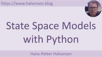
scipy.signal.lsimWe have the differential equations:1𝑥̇ ! 𝑥! 𝐾𝑢𝑇𝑥̇ " 0The State-space Model becomes:𝐾1𝑥𝑥̇ !! 𝑇 0 𝑥 𝑇 𝑢𝑥̇ ""0 00𝑦 1𝑥!0 𝑥"Here we use the following function:t, y, x sig.lsim(sys, u, t, x0)import scipy.signal as sigimport matplotlib.pyplot as pltimport numpy as np#Simulation Parametersx0 [0,0]start 0stop 30step 1t np.arange(start,stop,step)N len(t)u np.ones(N)K 3T 4# State-space ModelA [[-1/T, 0],[0, 0]]B [[K/T],[0]]C [[1, 0]]D 0sys sig.StateSpace(A, B, C, D)# Step Responset, y, x sig.lsim(sys, u, t)# Plottingplt.figure(1)plt.plot(t, y)plt.title("Step plt.show()# Alternatively you can plot one or more of the x variablesx1 x[:, 0]x2 x[:, 1]plt.figure(2)plt.plot(t, x1, t, x2)plt.title("Step Response")plt.xlabel("t")plt.ylabel("x1 and x2")plt.grid()plt.show()
ResultsPlotting 𝑦Plotting 𝑥! and 𝑥"
https://www.halvorsen.blogPython ControlSystems LibraryHans-Petter Halvorsen
Python Control Systems Library The Python Control Systems Library (control) is aPython package that implements basic operationsfor analysis and design of feedback control systems. Existing MATLAB user? The functions and thefeatures are very similar to the MATLAB ControlSystems Toolbox. Python Control Systems Library Homepage:https://pypi.org/project/control Python Control Systems Library o
InstallationThe Python Control Systems Librarypackage may be installed using pip:pip install control PIP is a Package Manager for Pythonpackages/modules. You find more information here:https://pypi.org Search for “control“. The Python Package Index (PyPI) is arepository of Python packages whereyou use PIP in order to install them
Anaconda PromptIf you have installed Python with Anaconda Distribution, use the Anaconda Prompt in orderto install it (just search for it using the Search field in Windows).pip install controlpip list
Command Prompt - PIPpip install on\Python37-32\Scripts\pip install controlpip listor “Python37 64“ for Python 64bits
Python Control Systems Library - FunctionsFunctions for Model Creation and Manipulation: tf()- Create a transfer function system ss()- Create a state space system c2d()- Return a discrete-time system tf2ss()- Transform a transfer function to a state space system ss2tf()- Transform a state space system to a transfer function Functions for Model Simulations: step response()- Step response of a linear system (e.g., a Statespace Model) lsim()- Simulate the output of a linear system (e.g., a State-spaceModel)
Python Example𝑥̇ 0 1 𝑥 0 𝑢𝑥𝑥̇ 0 1 1𝑥 𝑦 1 0 𝑥 import controlA [[0, 1],[0, -1]]B [[0],[1]]C [[1, 0]]D 0sys control.ss(A, B, C, D)
Step ResponseHere we use the following function:T,yout step response(sys, T, X0)State-space Model:𝑥̇ 01 𝑥 1 𝑢𝑥𝑥̇ 1 3 0𝑥 𝑦 5 6 𝑥 1𝑢 import controlimport matplotlib.pyplot as plt#ABCDDefine State-space Model [[0, 1], [-1, -3]] [[1], [0]] [[5, 6]] [[1]]ssmodel control.ss(A, B, C, D)# Step response for the systemt, y control.step response(ssmodel)plt.plot(t, y)plt.title("Step plt.show()This function uses the forced response() function with the input set to a unit step
Step Responseimport matplotlib.pyplot as pltimport controlState-space Model:𝑥̇ 0 𝑥̇ % 1𝑦 51 𝑥 0 3 𝑥%2𝑥 6 𝑥 7%Code Not Working!!!!!0 𝑢 4 𝑢%𝑢 0 𝑢%#ABCDDefine [[0, [[0, [[5, [[7,State-space Model1], [-1, -3]]0], [2, 4]]6]]0]]ssmodel control.ss(A, B, C, D)print(ssmodel)t, y control.step response(ssmodel)plt.plot(t, y)Note! This is a MISO system (Multiple Input/SingleOutput). So, the Solution is to split it into 2 systems,one for 𝑢! and one for 𝑢" . Se next slides.A similar code will work with MATLAB,and we will get 2 plots, but the PythonControl package does not support that
Step Response1 (𝑢! )State-space Model:𝑥̇ !0 𝑥̇ " 1𝑦 51 𝑥!0 𝑢 3 𝑥"2 !𝑥!6 𝑥 7 𝑢!"We can also plot both 𝑥! and 𝑥" :x1 x[0 ,:]x2 x[1 ,:]plt.plot(t, x1, t, x2)import matplotlib.pyplot as pltimport control#ABCDDefine State-space Model [[0, 1], [-1, -3]] [[0], [2]] [[5, 6]] [7]ssmodel control.ss(A, B, C, D)print(ssmodel)t, y control.step response(ssmodel)plt.plot(t, y)
Step Response2 (𝑢" )State-space Model:1 𝑥!0 𝑢 3 𝑥"4 "𝑥̇ !0 𝑥̇ " 1𝑦 5import matplotlib.pyplot as pltimport control𝑥!6 𝑥 0 𝑢""We can also plot both 𝑥! and 𝑥" :x1 x[0 ,:]x2 x[1 ,:]plt.plot(t, x1, t, x2)#ABCDDefine State-space Model [[0, 1], [-1, -3]] [[0], [4]] [[5, 6]] [0]ssmodel control.ss(A, B, C, D)print(ssmodel)t, y control.step response(ssmodel)plt.plot(t, y)
https://www.halvorsen.blogState Space Modelsand Transfer FunctionsHans-Petter Halvorsen
ence/signal.html
Transfer FunctionsA general Transfer function is on the form:𝑦(𝑠)𝐻 𝑠 𝑢(𝑠)Where 𝑦 is the output and 𝑢 is the input and 𝑠 is the Laplace operator𝑢(𝑠)𝐻 𝑠𝑦(𝑠)It is recommended that you know about Transfer Functions. If not, take a closer look atmy Tutorial “Transfer Functions with Python”
SISO/MIMO SystemsWe have 4 different Types of Systems: SISO – Single Input/Single Output MISO – Multiple Input/Single Output SIMO – Single Input/Multiple Output MIMO – Multiple Input/Multiple Output
SciPy LibrarySISOimport scipy.signal as signalimport matplotlib.pyplot as plt1 𝑥/1 𝑢 3 𝑥00B [[1],[0]]Single Input/Single OutputState-space Model:𝑥̇ /0 𝑥̇ 0 1𝑦 1# SISO System# Define State-space ModelA [[0, 1],[-1, -3]]C [[1, 0]]𝑥/0 𝑥 2𝑢0D [[2]]# Find Transfer Function from u to ynum, den signal.ss2tf(A, B, C, D)H signal.TransferFunction(num, den)print(H)𝑦𝑢𝐻(𝑠) 𝑦(𝑠)𝑢(𝑠)# Step response for the systemt, y signal.step(H)plt.plot(t, y)plt.title("Step Response w()
Control LibrarySISOimport controlimport matplotlib.pyplot as plt1 𝑥/1 𝑢 3 𝑥00B [[1],[0]]Single Input/Single OutputState-space Model:𝑥̇ /0 𝑥̇ 0 1𝑦 1# SISO System# Define State-space ModelA [[0, 1],[-1, -3]]C [[1, 0]]𝑥/0 𝑥 2𝑢0D [[2]]ssmodel control.ss(A, B, C, D)𝑦𝑢H control.ss2tf(ssmodel)print(H)# Step response for the systemt, y control.step response(H)𝐻(𝑠) 𝑦(𝑠)𝑢(𝑠)plt.plot(t, y)plt.title("Step Response w()
import scipy.signal as signalimport matplotlib.pyplot as pltMISOSciPy LibraryState-space Model:𝑥̇ /0 𝑥̇ 0 1Multiple Input/Single OutputB [[0, 0],[2, 4]]1 𝑥/0 3 𝑥02𝑦 1𝑢!𝑢"𝑦(𝑠)𝐻! (𝑠) 𝑢! (𝑠)# MISO System# Define State-space ModelA [[0, 1],[-1, -3]]0 𝑢/4 𝑢0C [[1, 0]]D [[0, 0]]𝑥/0 𝑥0# Find Transfer Function from u1 to ynum, den signal.ss2tf(A, B, C, D, 0)H1 signal.TransferFunction(num, den)print(H1)𝑦𝑦(𝑠)𝐻" (𝑠) 𝑢" (𝑠)# Find Transfer Function from u2 to ynum, den signal.ss2tf(A, B, C, D, 1)H2 signal.TransferFunction(num, den)print(H2)# Step response for the systemt, y signal.step(H1)plt.plot(t, y)t, y signal.step(H2)plt.plot(t, y)plt.title("Step (["H1", "H2"])plt.grid()
MISOControl LibraryState-space Model:𝑥̇ /0 𝑥̇ 0 1import controlimport matplotlib.pyplot as pltMultiple Input/Single OutputB [[0, 0],[2, 4]]1 𝑥/0 3 𝑥02𝑦 1𝑢!𝑢"# MISO System# Define State-space ModelA [[0, 1],[-1, -3]]0 𝑢/4 𝑢0𝑥/0 𝑥0C [[1, 0]]D 0ssmodel control.ss(A, B, C, D)H control.ss2tf(ssmodel)print(H)H1 H[0,0]print(H1)H2 H[0,1]print(H2)𝑦# Step response for the systemt, y control.step response(H1)plt.plot(t, y)t, y control.step response(H2)plt.plot(t, y)𝑦(𝑠)𝐻! (𝑠) 𝑢! (𝑠)𝑦(𝑠)𝐻" (𝑠) 𝑢" (𝑠)plt.title("Step (["H1", "H2"])plt.grid()plt.show()
SciPy Libraryimport scipy.signal as signalimport matplotlib.pyplot as pltSIMOState-space Model:𝑥̇ /0 𝑥̇ 0 1Single Input/Multiple OutputB [[0],[2]]C [[1, 0],[0, 1]]1 𝑥/0 𝑢𝑥 3 02𝑦/1𝑦 𝑦 00𝑢# SIMO System# Define State-space ModelA [[0, 1],[-1, -3]]D [[0]]# Find Transfer Function from u to y1C [[1, 0]]num, den signal.ss2tf(A, B, C, D)H1 signal.TransferFunction(num, den)print(H1)0 𝑥/1 𝑥0𝑦!# Find Transfer Function from u to y2C [[0, 1]]num, den signal.ss2tf(A, B, C, D)H2 signal.TransferFunction(num, den)print(H2)𝑦"# Step response for the systemt, y signal.step(H1)plt.plot(t, y)t, y signal.step(H2)plt.plot(t, y)𝑦! (𝑠)𝐻! (𝑠) 𝑢(𝑠)𝑦" (𝑠)𝐻" (𝑠) 𝑢(𝑠)plt.title("Step (["H1", "H2"])plt.grid()plt.show()
Control Libraryimport controlimport matplotlib.pyplot as pltSIMOState-space Model:𝑥̇ /0 𝑥̇ 0 1Single Input/Multiple OutputB [[0],[2]]C [[1, 0],[0, 1]]1 𝑥/0 𝑢𝑥 3 02𝑦/1𝑦 𝑦 00𝑢# SIMO System# Define State-space ModelA [[0, 1],[-1, -3]]D 0ssmodel control.ss(A, B, C, D)0 𝑥/1 𝑥0𝑦!𝑦"H control.ss2tf(ssmodel)print(H)H1 H[0,0]print(H1)H2 H[1,0]print(H2)# Step response for the systemt, y control.step response(H)y1 y[0, :]y2 y[1, :]plt.plot(t, y1)plt.plot(t, y2)𝑦! (𝑠)𝐻! (𝑠) 𝑢(𝑠)𝑦" (𝑠)𝐻" (𝑠) 𝑢(𝑠)plt.title("Step (["H1", "H2"])plt.grid()plt.show()
MIMOSciPy LibraryState-space Model:𝑥̇ /0 𝑥̇ 0 1import scipy.signal as signalimport matplotlib.pyplot as plt# SIMO System# Define State-space ModelA [[0, 1],[-1, -3]]Multiple Input/Multiple OutputD [[0, 0]]1 𝑥/0 3 𝑥02𝑦/1𝑦 𝑦 000 𝑢/4 𝑢0𝑦!𝑢"𝑦"𝑦! (𝑠)𝑢! (𝑠)𝑦" (𝑠)𝐻% (𝑠) 𝑢! (𝑠)𝐻" (𝑠) C [[1, 0]]# Find Transfer Function from u1 to y1num, den signal.ss2tf(A, B, C, D, 0)H1 signal.TransferFunction(num, den)print(H1)# Find Transfer Function from u2 to y1num, den signal.ss2tf(A, B, C, D, 1)H2 signal.TransferFunction(num, den)print(H2)0 𝑥/1 𝑥0𝑢!𝐻! (𝑠) B [[0, 0],[2, 4]]𝑦! (𝑠)𝑢" (𝑠)𝑦" (𝑠)𝐻& (𝑠) 𝑢" (𝑠)C [[0, 1]]# Find Transfer Function from u1 to y2num, den signal.ss2tf(A, B, C, D, 0)H3 signal.TransferFunction(num, den)print(H3)# Find Transfer Function from u1 to y2num, den signal.ss2tf(A, B, C, D, 1)H4 signal.TransferFunction(num, den)print(H4)# Step response for the systemt, y signal.step(H1)plt.plot(t, y)t, y signal.step(H2)plt.plot(t, y)t, y signal.step(H3)plt.plot(t, y)t, y signal.step(H4)plt.plot(t, y)plt.title("Step (["H1", "H2", "H3", "H4"])plt.grid()plt.show()
MIMOControl LibraryState-space Model:𝑥̇ /0 𝑥̇ 0 1import controlimport matplotlib.pyplot as pltMultiple Input/Multiple Output1 𝑥/0 3 𝑥02𝑦/1𝑦 𝑦 000 𝑢/4 𝑢00 𝑥/1 𝑥0# MIMO System# Define State-space ModelA [[0, 1],[-1, -3]]B [[0, 0],[2, 4]]C [[1, 0],[0, 1]]D 0ssmodel control.ss(A, B, C, D)𝑢!𝑦!H control.ss2tf(ssmodel)print(H)H1 H[0,0]print(H1)H2 H[0,1]print(H2)H3 H[1,0]print(H3)H4 H[1,1]print(H4)𝑢"𝑦"# Step response for the systemt, y control.step response(H1)plt.plot(t, y)𝐻! (𝑠) 𝑦! (𝑠)𝑢! (𝑠)𝑦" (𝑠)𝐻% (𝑠) 𝑢! (𝑠)𝐻" (𝑠) 𝑦! (𝑠)𝑢" (𝑠)𝑦" (𝑠)𝐻& (𝑠) 𝑢" (𝑠)t, y control.step response(H2)plt.plot(t, y)t, y control.step response(H3)plt.plot(t, y)t, y control.step response(H4)plt.plot(t, y)plt.title("Step Response H")plt.xlabel("t")plt.ylabel("y")plt.legend(["H1", "H2", "H3", "H4"])plt.grid()plt.show()
https://www.halvorsen.blogDiscrete State SpaceModelsHans-Petter Halvorsen
Discretization Methods EulerWe have many different Discretization Methods–Euler forward method–Euler backward methodWe will focus on thissince it it easy to useand implement Zero Order Hold (ZOH) TustinIt is recommended that you know about Discrete Systems. If not, .take a closer look at my Tutorial “Discrete Systems with Python”
Discretization MethodsEuler forward method:𝑥 𝑘 1 𝑥(𝑘)𝑥̇ 𝑇(Where 𝑇' is the sampling time, and 𝑥(𝑘 1), 𝑥(𝑘) and 𝑥(𝑘 1) are discrete values of 𝑥(𝑡)
Discretization ExampleDifferential Equation (1.order system):1!)or:𝑥̇ 𝑥 𝑢𝑥̇ 𝑥 𝐾𝑢((𝑇We use Euler forward method:𝑥̇ 𝑥 𝑘 1 𝑥(𝑘)𝑇'Then we get:𝑥 𝑘 1 𝑥(𝑘)1𝐾 𝑥(𝑘) 𝑢(𝑘)𝑇'𝑇𝑇Further:𝑥 𝑘 1 𝑥 𝑘 𝑇'1𝐾 𝑥(𝑘) 𝑢(𝑘)𝑇𝑇And:𝑇'𝑇' 𝐾𝑥 𝑘 1 𝑥 𝑘 𝑥 𝑘 𝑢(𝑘)𝑇𝑇Finally:𝑥 𝑘 1 1 𝑇'𝑇' 𝐾𝑥 𝑘 𝑢(𝑘)𝑇𝑇
Discrete State-space ModelsGiven a Continuous State-space Model:𝑥̇ 𝐴𝑥 𝐵𝑢𝑦 𝐶𝑥 𝐷𝑢The Discrete State-space Model is then given by:𝑥34! 𝐼 𝑇5 𝐴 𝑥3 𝑇5 𝐵𝑢3𝑦3 𝐶𝑥3 𝐷𝑢3This equation is derived using the Euler forwardmethod on a general state-space model.𝑇' is the discrete Sampling Time𝑥* ! 𝐴, 𝑥* 𝐵, 𝑢*𝑦* 𝐶, 𝑥* 𝐷, 𝑢*
ence/signal.html
Discrete State-space ModelsGiven the following:We have the differential equations:1𝑥̇ ! 𝑥! 𝐾𝑢𝑇𝑥̇ " 0What is the discrete State-space Model?The State-space Model becomes:𝐾0 𝑥 𝑇 𝑢𝑥%00𝑥 𝑦 1 0 𝑥%1𝑥̇ 𝑇𝑥̇ %0
Discrete State-space ModelsWe have the differential equations:1𝑥̇ ! 𝑥! 𝐾𝑢𝑇𝑥̇ " 0We use Euler forward method:𝑥̇ 𝑥 𝑘 1 𝑥(𝑘)𝑇'𝑥" 𝑘 1 𝑥" 𝑘 0𝑇'𝑥" 𝑘 1 𝑥" 𝑘𝑥! 𝑘 1 1 𝑇'𝑇' 𝐾𝑥! 𝑘 𝑢(𝑘)𝑇𝑇𝑥" 𝑘 1 𝑥" 𝑘This gives the following Discrete State-space model:𝑥! 𝑘 1𝑥" 𝑘 1 𝑇'1 𝑇0𝑦(𝑘) 10 𝑥! 𝑘𝑥 𝑘1 "0𝑥! 𝑘𝑥" 𝑘𝑇' 𝐾 𝑇 𝑢(𝑘)0
Discrete State-space ModelsDiscrete State-space model:𝑥! 𝑘 1𝑥" 𝑘 1 𝑇'1 𝑇0𝑦(𝑘) 10 𝑥! 𝑘𝑥 𝑘1 "0𝑇' 𝐾 𝑇 𝑢(𝑘)0𝑥! 𝑘𝑥" 𝑘We set 𝐾 3, 𝑇 4𝑇' 0.1𝑥! 𝑘 1𝑥" 𝑘 1 0.9750𝑦(𝑘) 10 𝑥! 𝑘1 𝑥" 𝑘0𝑥! 𝑘𝑥" 𝑘 0.075𝑢(𝑘)0
Python Exampleimport scipy.signal as sigK 3T 4# State-space ModelA [[-1/T, 0],[0, 0]]B [[K/T],[0]]C [[1, 0]]D 0sys sig.StateSpace(A, B, C, D)print(sys)sys d sys.to discrete(dt 0.1, method 'euler')print(sys d)StateSpaceContinuous(array([[-0.25, 0. ],[ 0. , 0. ]]),array([[0.75],[0. ]]),array([[1, 0]]),array([[0]]),dt: None)StateSpaceDiscrete(array([[0.975, 0.],[0., 1.]]),array([[0.075],[0.]]),array([[1., 0.]]),array([[0.]]),dt: 0.1)We see that weget the correctanswer
Python ExampleImplement Discretization from scratch𝑥JK 𝐼 𝑇L 𝐴 𝑥J 𝑇L 𝐵𝑢J𝑦J 𝐶𝑥J 𝐷𝑢Jimport numpy as npimport scipy.signal as sigK 3T 4# State-space ModelA np.array([[-1/T, 0], [0, 0]])B np.array([[K/T], [0]])C np.array([[1, 0]])D 0sys sig.StateSpace(A, B, C, D)sys d sys.to discrete(dt 0.1, method 'euler')print(sys d)I np.eye(len(A[0]))𝐴, 𝐼 𝑇' 𝐴𝐵, 𝑇' 𝐵Ts 0.1Ad I Ts * Aprint(Ad)Bd Ts * Bprint(Bd)sys d2 sig.StateSpace(Ad, Bd, C, D, dt Ts)print(sys d)
Python ExampleImplement self-made c2d() function𝑥JK 𝐼 𝑇L 𝐴 𝑥J 𝑇L 𝐵𝑢J𝑦J 𝐶𝑥J 𝐷𝑢Jimport numpy as npimport scipy.signal as sigdef c2d(A,B, Ts):I np.eye(len(A[0]))Ts 0.1Ad I Ts * ABd Ts * Breturn Ad, BdK 3T 4# State-space ModelA np.array([[-1/T, 0], [0, 0]])B np.array([[K/T], [0]])𝐴, 𝐼 𝑇' 𝐴C np.array([[1, 0]])D 0𝐵, 𝑇' 𝐵Ts 0.1Ad, Bd c2d(A, B, Ts)sys d sig.StateSpace(Ad, Bd, C, D, dt Ts)print(sys d)
https://www.halvorsen.blogMass-Spring-DamperSystem with PythonHans-Petter Halvorsen
Mass-Spring-Damper SystemThe ”Mass-Spring-Damper“ System istypical system used to demonstrate andillustrate Modelling and 𝑥(𝑡)𝑐Damper
Mass-Spring-Damper SystemGiven a so-called "Mass-Spring-Damper" systemNewtons 2.law: 𝐹 𝑚𝑎The system can be described by the following equation:𝐹 𝑡 𝑐 𝑥̇ 𝑡 𝑘𝑥 𝑡 𝑚𝑥(𝑡)̈Where 𝑡 is the time, 𝐹(𝑡) is an external force applied to the system, 𝑐 is thedamping constant, 𝑘 is the stiffness of the spring, 𝑚 is a mass.𝑥(𝑡) is the position of the object (𝑚)𝑥̇ 𝑡 is the first derivative of the position, which equals the velocity/speedof the object (𝑚)𝑥(𝑡)̈is the second derivative of the position, which equals the accelerationof the object (𝑚)
Mass-Spring-Damper System𝐹 𝑡 𝑐𝑥̇ 𝑡 𝑘𝑥 𝑡 𝑚𝑥(𝑡)̈𝑚𝑥̈ 𝐹 𝑐𝑥̇ 𝑘𝑥1𝑥̈ 𝐹 𝑐𝑥̇ 𝑘𝑥𝑚We set𝑥 𝑥!𝑥̇ 𝑥"Higher order differential equations can typicallybe reformulated into a system of first orderdifferential equationsThis gives:𝑥̇ ! 𝑥"!𝑥̇ " 𝑥 ̈𝐹 𝑐𝑥̇ 𝑘𝑥 Finally:1𝑥̈ 𝐹 𝑐 𝑥̇ 𝑘𝑥𝑚 𝑥! Position𝑥" Velocity/Speed! 𝐹 𝑐𝑥" 𝑘𝑥!𝑥̇ 𝑥 𝑥̇ R 𝐹 𝑐𝑥 𝑘𝑥
State-space Model𝑥̇ 𝑥 𝑥̇ R 𝐹 𝑐𝑥 𝑘𝑥 𝑥̇ 𝑥 JS 𝑥̇ R 𝑥 R 𝑥 R 𝐹𝑥̇ 𝐴𝑥 𝐵𝑢0𝑥̇ 𝑘 𝑥̇ 𝑚𝑥̇ 𝐴𝑥 𝐵𝑢0𝑘𝐴 𝑚1𝑐 𝑚0𝐵 1𝑚𝑥 𝑥 𝑥%𝐹 𝑢10𝑥 1 𝐹𝑐 𝑥 𝑚𝑚
Python CodeState-space Model0𝑥̇ !𝑘 𝑥̇ " 𝑚𝑦 110𝑥!𝑐 1 𝐹𝑥 "𝑚𝑚𝑥!0 𝑥"import numpy as npimport matplotlib.pyplot as pltimport scipy.signal as sig# Parameters defining the systemc 4 # Damping constantk 2 # Stiffness of the springm 20 # MassF 5 # ForceFt np.ones(610)*F# Simulation Parameterststart 0tstop 60increment 0.1t np.arange(tstart,tstop 1,increment)# System matricesA [[0, 1], [-k/m, -c/m]]B [[0], [1/m]]C [[1, 0]]sys sig.StateSpace(A, B, C, 0)# Step response for the systemt, y, x sig.lsim(sys, Ft, t)x1 x[:,0]x2 x[:,1]plt.plot(t, x1, t, x2)#plt.plot(t, y)plt.title('Simulation of Mass-Spring-Damper )plt.show()
Python Control Systems Library - FunctionsFunctions for Model Creation and Manipulation: tf()- Create a transfer function system ss()- Create a state space system c2d()- Return a discrete-time system tf2ss()- Transform a transfer function to a state space system ss2tf()- Transform a state space system to a transfer function Functions for Model Simulations: step response()- Step response of a linear system forced response() lsim()- Simulate the output of a linear system
Python CodeState-space Model0𝑥̇ !𝑘 𝑥̇ " 𝑚𝑦 110𝑥!𝑐 1 𝐹𝑥 "𝑚𝑚𝑥!0 𝑥"import numpy as npimport matplotlib.pyplot as pltimport control#ckmFParameters defining the system 4 # Damping constant 2 # Stiffness of the spring 20 # Mass 5 # Force# Simulation Parameterststart 0tstop 60increment 0.1t np.arange(tstart,tstop 1,increment)# System matricesA [[0, 1], [-k/m, -c/m]]B [[0], [1/m]]C [[1, 0]]D 0sys control.ss(A, B, C, D)# Step response for the systemt, y, x control.forced response(sys, t, F)plt.plot(t, y)plt.title('Simulation of Mass-Spring-Damper System')plt.xlabel('t’); plt.ylabel('x(t)')plt.grid()plt.show()
Python CodeState-space Model0𝑥̇ !𝑘 𝑥̇ " 𝑚𝑦 110𝑥!𝑐 1 𝐹𝑥 "𝑚𝑚𝑥!0 𝑥"import numpy as npimport matplotlib.pyplot as pltimport control#ckmFParameters defining the system 4 # Damping constant 2 # Stiffness of the spring 20 # Mass 5 # Force# Simulation Parameterststart 0tstop 60increment 0.1t np.arange(tstart,tstop 1,increment)# System matricesA [[0, 1], [-k/m, -c/m]]B [[0], [1/m]]C [[1, 0]]D 0sys control.ss(A, B, C, D)# Step response for the systemt, y, x control.forced response(sys, t, F)x1 x[0 ,:]x2 x[1 ,:]plt.plot(t, x1, t, x2)plt.title('Simulation of Mass-Spring-Damper )plt.show()
DiscretizationGiven:𝑥̇ " !#𝑥̇ ! 𝑥"𝐹 𝑐𝑥" 𝑘𝑥!%&!𝑥" 𝑘 1 𝑇 # 𝑥! 𝑘 𝑥" 𝑘 𝑇 # 𝑥" 𝑘 𝑇 # 𝐹(𝑘)Using Euler:𝑥̇ 𝑥 𝑘 1 𝑥(𝑘)𝑇 Then we get:𝑥! 𝑘 1 𝑥! 𝑘 𝑥" 𝑘𝑇 𝑥" 𝑘 1 𝑥" 𝑘1 𝐹(𝑘) 𝑐𝑥" 𝑘 𝑘𝑥! 𝑘𝑇 𝑚This gives:Then we get:𝑥! 𝑘 1 𝑥! 𝑘 𝑇 𝑥" 𝑘𝑥! 𝑘 1 𝑥! 𝑘 𝑇 𝑥" 𝑘1𝑥" 𝑘 1 𝑥" 𝑘 𝑇 𝐹(𝑘) 𝑐𝑥" 𝑘 𝑘𝑥! 𝑘𝑚Finally:𝑥! 𝑘 1 𝑥! 𝑘 𝑇 𝑥" 𝑘%&!𝑥" 𝑘 1 𝑇 # 𝑥! 𝑘 (1 𝑇 #)𝑥" 𝑘 𝑇 # 𝐹(𝑘)
Discrete State-space ModelDiscrete System:𝑥! 𝑘 1 𝑥! 𝑘 𝑇' 𝑥" 𝑘*𝑥" 𝑘 1 𝑇' 𝑥! 𝑘 (1 𝑇' )𝑥" 𝑘 𝑇' 1! 𝐹(𝑘)𝐴 𝑘 𝑇'𝑚𝑇'𝑐1 𝑇'𝑚We can set it on Discrete state space form:01𝐵 𝑇'𝑚𝑥(𝑘 1) 𝐴, 𝑥(𝑘) 𝐵, 𝑢(𝑘)This gives:𝑥! 𝑘 1𝑥" 𝑘 11 𝑘 𝑇'𝑚𝑇'𝑐1 𝑇'𝑚𝑥! 𝑘𝑥" 𝑘01 𝐹(𝑘) 𝑇'𝑚𝑥(𝑘) 𝑥 𝑘𝑥% 𝑘We can also use control.c2d() function
Python Code# Simulation of Mass-Spring-Damper Systemimport numpy as npimport matplotlib.pyplot as pltDiscrete System𝑥! 𝑘 1 𝑥! 𝑘 𝑇' 𝑥" 𝑘*𝑥" 𝑘 1 𝑇' 𝑥! 𝑘 (1 𝑇' )𝑥" 𝑘 𝑇' 𝑥! Position𝑥" Velocity/Speed ! 𝐹(𝑘)#ckmFModel Parameters 4 # Damping constant 2 # Stiffness of the spring 20 # Mass 5 # Force# Simulation ParametersTs 0.1Tstart 0Tstop 60N int((Tstop-Tstart)/Ts) # Simulation lengthx1 np.zeros(N 2)x2 np.zeros(N 2)x1[0] 0 # Initial Positionx2[0] 0 # Initial Speeda11a12a21a22 1Ts-(Ts*k)/m1 - (Ts*c)/mb1 0b2 Ts/m# Simulationfor k in range(N 1):x1[k 1] a11 * x1[k] a12 * x2[k] b1 * Fx2[k 1] a21 * x1[k] a22 * x2[k] b2 * F# Plot the Simulation Resultst np.arange(Tstart,Tstop 2*Ts,Ts)#plt.plot(t, x1, t, on of Mass-Spring-Damper System')plt.xlabel('t [s]')plt.ylabel('x(t)')plt.grid()plt.legend(["x1", "x2"])plt.show()
Additional Python ramming/python/
Hans-Petter HalvorsenUniversity of South-Eastern Norwaywww.usn.noE-mail: hans.p.halvorsen@usn.noWeb: https://www.halvorsen.blog
Python Examples -SciPy (SciPy.signal) -The Python Control Systems Library Contents It is recommended that you know about Vectors, Matrices and Linear Algebra. If not, take a closer look at my Tutorial "Linear Algebra with Python". You should also know about differential equations, see "Differential Equations in Python"