WIXLIB

1.3How Supervised Learning WorksIn this section, I briefly explain how supervised learning works so that you have the pictureof the whole process before we go into detail. I decided to use supervised learning as anexample because it’s the type of machine learning most frequently used in practice.The supervised learning process starts with gathering the data. The data for supervisedlearning is a collection of pairs (input, output). Input could be anything, for example, emailmessages, pictures, or sensor measurements. Outputs are usually real numbers, or labels (e.g.“spam”, “not spam”, “cat”, “dog”, “mouse”, etc). In some cases, outputs are vectors (e.g.,four coordinates of the rectangle around a person on the picture), sequences (e.g. [“adjective”,“adjective”, “noun”] for the input “big beautiful car”), or have some other structure.Let’s say the problem that you want to solve using supervised learning is spam detection.You gather the data, for example, 10,000 email messages, each with a label either “spam” or“not spam” (you could add those labels manually or pay someone to do that for us). Now,you have to convert each email message into a feature vector.The data analyst decides, based on their experience, how to convert a real-world entity, suchas an email message, into a feature vector. One common way to convert a text into a featurevector, called bag of words, is to take a dictionary of English words (let’s say it contains20,000 alphabetically sorted words) and stipulate that in our feature vector: the first feature is equal to 1 if the email message contains the word “a”; otherwise,this feature is 0; the second feature is equal to 1 if the email message contains the word “aaron”; otherwise,this feature equals 0; . the feature at position 20,000 is equal to 1 if the email message contains the word“zulu”; otherwise, this feature is equal to 0.You repeat the above procedure for every email message in our collection, which givesus 10,000 feature vectors (each vector having the dimensionality of 20,000) and a label(“spam”/“not spam”).Now you have a machine-readable input data, but the output labels are still in the form ofhuman-readable text. Some learning algorithms require transforming labels into numbers.For example, some algorithms require numbers like 0 (to represent the label “not spam”)and 1 (to represent the label “spam”). The algorithm I use to illustrate supervised learning iscalled Support Vector Machine (SVM). This algorithm requires that the positive label (inour case it’s “spam”) has the numeric value of 1 (one), and the negative label (“not spam”)has the value of 1 (minus one).At this point, you have a dataset and a learning algorithm, so you are ready to applythe learning algorithm to the dataset to get the model.SVM sees every feature vector as a point in a high-dimensional space (in our case, spaceAndriy BurkovThe Hundred-Page Machine Learning Book - Draft5

is 20,000-dimensional). The algorithm puts all feature vectors on an imaginary 20,000dimensional plot and draws an imaginary 20,000-dimensional line (a hyperplane) that separatesexamples with positive labels from examples with negative labels. In machine learning, theboundary separating the examples of different classes is called the decision boundary.The equation of the hyperplane is given by two parameters, a real-valued vector w of thesame dimensionality as our input feature vector x, and a real number b like this:wx b 0,where the expression wx means w(1) x(1) w(2) x(2) . . . w(D) x(D) , and D is the numberof dimensions of the feature vector x.(If some equations aren’t clear to you right now, in Chapter 2 we revisit the math andstatistical concepts necessary to understand them. For the moment, try to get an intuition ofwhat’s happening here. It all becomes more clear after you read the next chapter.)Now, the predicted label for some input feature vector x is given like this:y sign(wx b),where sign is a mathematical operator that takes any value as input and returns 1 if theinput is a positive number or 1 if the input is a negative number.The goal of the learning algorithm — SVM in this case — is to leverage the dataset and findthe optimal values wú and bú for parameters w and b. Once the learning algorithm identifiesthese optimal values, the model f (x) is then defined as:f (x) sign(wú x bú )Therefore, to predict whether an email message is spam or not spam using an SVM model,you have to take a text of the message, convert it into a feature vector, then multiply thisvector by wú , subtract bú and take the sign of the result. This will give us the prediction ( 1means “spam”, 1 means “not spam”).Now, how does the machine find wú and bú ? It solves an optimization problem. Machinesare good at optimizing functions under constraints.So what are the constraints we want to satisfy here? First of all, we want the model to predictthe labels of our 10,000 examples correctly. Remember that each example i 1, . . . , 10000 isgiven by a pair (xi , yi ), where xi is the feature vector of example i and yi is its label thattakes values either 1 or 1. So the constraints are naturally: wxi b Ø 1 if yi 1, and wxi b Æ 1 if yi 1Andriy BurkovThe Hundred-Page Machine Learning Book - Draft6

1x(2)2wx—b —1wx—b 0wx—b w w bx(1)Figure 1: An example of an SVM model for two-dimensional feature vectors.We would also prefer that the hyperplane separates positive examples from negative ones withthe largest margin. The margin is the distance between the closest examples of two classes,as defined by the decision boundary. A large margin contributes to a better generalization,that is how well the model will classify new examples in the future. ToÒachieve that, we needqD(j) )2 .to minimize the Euclidean norm of w denoted by ÎwÎ and given byj 1 (wSo, the optimization problem that we want the machine to solve looks like this:Minimize ÎwÎ subject to yi (wxi b) Ø 1 for i 1, . . . , N . The expression yi (wxi b) Ø 1is just a compact way to write the above two constraints.The solution of this optimization problem, given by wú and bú , is called the statisticalmodel, or, simply, the model. The process of building the model is called training.For two-dimensional feature vectors, the problem and the solution can be visualized as shownin fig. 1. The blue and orange circles represent, respectively, positive and negative examples,and the line given by wx b 0 is the decision boundary.Why, by minimizing the norm of w, do we find the highest margin between the two classes?Geometrically, the equations wx b 1 and wx b 1 define two parallel hyperplanes,2as you see in fig. 1. The distance between these hyperplanes is given by ÎwÎ, so the smallerAndriy BurkovThe Hundred-Page Machine Learning Book - Draft7

the norm ÎwÎ, the larger the distance between these two hyperplanes.That’s how Support Vector Machines work. This particular version of the algorithm buildsthe so-called linear model. It’s called linear because the decision boundary is a straight line(or a plane, or a hyperplane). SVM can also incorporate kernels that can make the decisionboundary arbitrarily non-linear. In some cases, it could be impossible to perfectly separatethe two groups of points because of noise in the data, errors of labeling, or outliers (examplesvery different from a “typical” example in the dataset). Another version of SVM can alsoincorporate a penalty hyperparameter for misclassification of training examples of specificclasses. We study the SVM algorithm in more detail in Chapter 3.At this point, you should retain the following: any classification learning algorithm thatbuilds a model implicitly or explicitly creates a decision boundary. The decision boundarycan be straight, or curved, or it can have a complex form, or it can be a superposition ofsome geometrical figures. The form of the decision boundary determines the accuracy ofthe model (that is the ratio of examples whose labels are predicted correctly). The form ofthe decision boundary, the way it is algorithmically or mathematically computed based onthe training data, differentiates one learning algorithm from another.In practice, there are two other essential differentiators of learning algorithms to consider:speed of model building and prediction processing time. In many practical cases, you wouldprefer a learning algorithm that builds a less accurate model fast. Additionally, you mightprefer a less accurate model that is much quicker at making predictions.1.4Why the Model Works on New DataWhy is a machine-learned model capable of predicting correctly the labels of new, previouslyunseen examples? To understand that, look at the plot in fig. 1. If two classes are separablefrom one another by a decision boundary, then, obviously, examples that belong to each classare located in two different subspaces which the decision boundary creates.If the examples used for training were selected randomly, independently of one another, andfollowing the same procedure, then, statistically, it is more likely that the new negativeexample will be located on the plot somewhere not too far from other negative examples.The same concerns the new positive example: it will likely come from the surroundings ofother positive examples. In such a case, our decision boundary will still, with high probability,separate well new positive and negative examples from one another. For other, less likelysituations, our model will make errors, but because such situations are less likely, the numberof errors will likely be smaller than the number of correct predictions.Intuitively, the larger is the set of training examples, the more unlikely that the new exampleswill be dissimilar to (and lie on the plot far from) the examples used for training. To minimizethe probability of making errors on new examples, the SVM algorithm, by looking for thelargest margin, explicitly tries to draw the decision boundary in such a way that it lies as faras possible from examples of both classes.Andriy BurkovThe Hundred-Page Machine Learning Book - Draft8

The reader interested in knowing more about the learnability and understanding the close relationship between the model error, the size ofthe training set, the form of the mathematical equation that definesthe model, and the time it takes to build the model is encouraged toread about the PAC learning. The PAC (for “probably approximatelycorrect”) learning theory helps to analyze whether and under whatconditions a learning algorithm will probably output an approximatelycorrect classifier.Andriy BurkovThe Hundred-Page Machine Learning Book - Draft9

TheHundredPageMachineLearningBookAndriy Burkov

“All models are wrong, but some are useful.”— George BoxThe book is distributed on the “read first, buy later” principle.Andriy BurkovThe Hundred-Page Machine Learning Book - Draft

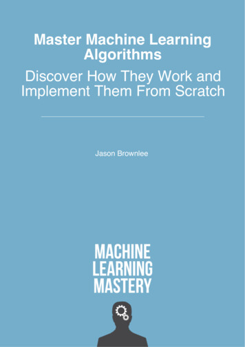
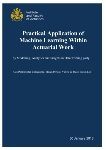
22.1Notation and DefinitionsNotationLet’s start by revisiting the mathematical notation we all learned at school, but some likelyforgot right after the prom.2.1.1Scalars, Vectors, and SetsA scalar is a simple numerical value, like 15 or 3.25. Variables or constants that take scalarvalues are denoted by an italic letter, like x or a.Figure 1: Three vectors visualized as directions and as points.A vector is an ordered list of scalar values, called attributes. We denote a vector as a boldcharacter, for example, x or w. Vectors can be visualized as arrows that point to somedirections as well as points in a multi-dimensional space. Illustrations of three two-dimensionalvectors, a [2, 3], b [ 2, 5], and c [1, 0] is given in fig. 1. We denote an attribute of avector as an italic value with an index, like this: w(j) or x(j) . The index j denotes a specificdimension of the vector, the position of an attribute in the list. For instance, in the vector ashown in red in fig. 1, a(1) 2 and a(2) 3.The notation x(j) should not be confused with the power operator, like this x2 (squared) orx3 (cubed). If we want to apply a power operator, say square, to an indexed attribute of avector, we write like this: (x(j) )2 .(j)A variable can have two or more indices, like this: xi(j)(k)or like this xi,j . For example, inneural networks, we denote as xl,u the input feature j of unit u in layer l.Andriy BurkovThe Hundred-Page Machine Learning Book - Draft3

A set is an unordered collection of unique elements. We denote a set as a calligraphiccapital character, for example, S. A set of numbers can be finite (include a fixed amountof values). In this case, it is denoted using accolades, for example, {1, 3, 18, 23, 235} or{x1 , x2 , x3 , x4 , . . . , xn }. A set can be infinite and include all values in some interval. If a setincludes all values between a and b, including a and b, it is denoted using brackets as [a, b].If the set doesn’t include the values a and b, such a set is denoted using parentheses like this:(a, b). For example, the set [0, 1] includes such values as 0, 0.0001, 0.25, 0.784, 0.9995, and1.0. A special set denoted R includes all numbers from minus infinity to plus infinity.When an element x belongs to a set S, we write x œ S. We can obtain a new set S3 asan intersection of two sets S1 and S2 . In this case, we write S3 Ω S1 fl S2 . For example{1, 3, 5, 8} fl {1, 8, 4} gives the new set {1, 8}.We can obtain a new set S3 as a union of two sets S1 and S2 . In this case, we writeS3 Ω S1 fi S2 . For example {1, 3, 5, 8} fi {1, 8, 4} gives the new set {1, 3, 4, 5, 8}.2.1.2Capital Sigma NotationThe summation over a collection X {x1 , x2 , . . . , xn 1 , xn } or over the attributes of a vectorx [x(1) , x(2) , . . . , x(m 1) , x(m) ] is denoted like this:nÿdefxi x1 x2 . . . xn 1 xn , or else:i 1mÿdefx(j) x(1) x(2) . . . x(m 1) x(m) .j 1defThe notation means “is defined as”.2.1.3Capital Pi NotationA notation analogous to capital sigma is the capital pi notation. It denotes a product ofelements in a collection or attributes of a vector:nŸi 1defxi x1 · x2 · . . . · xn 1 · xn ,where a · b means a multiplied by b. Where possible, we omit · to simplify the notation, so abalso means a multiplied by b.Andriy BurkovThe Hundred-Page Machine Learning Book - Draft4

2.1.4Operations on SetsA derived set creation operator looks like this: S Õ Ω {x2 x œ S, x 3}. This notation meansthat we create a new set S Õ by putting into it x squared such that that x is in S, and x isgreater than 3.The cardinality operator S returns the number of elements in set S.2.1.5Operations on VectorsThe sum of two vectors x z is defined as the vector [x(1) z (1) , x(2) z (2) , . . . , x(m) z (m) ].The difference of two vectors x z is defined as the vector [x(1) z (1) , x(2) z (2) , . . . , x(m) z (m) ].defA vector multiplied by a scalar is a vector. For example xc [cx(1) , cx(2) , . . . , cx(m) ].def qmA dot-product of two vectors is a scalar. For example, wx i 1 w(i) x(i) . In some books,the dot-product is denoted as w · x. The two vectors must be of the same dimensionality.Otherwise, the dot-product is undefined.The multiplication of a matrix W by a vector x gives another vector as a result. Let ourmatrix be,5 (1,1)wW w(2,1)w(1,2)w(2,2)6w(1,3).w(2,3)When vectors participate in operations on matrices, a vector is by default represented as amatrix with one column. When the vector is on the right of the matrix, it remains a columnvector. We can only multiply a matrix by vector if the vector has the same number of rowsdefas the number of columns in the matrix. Let our vector be x [x(1) , x(2) , x(3) ]. Then Wxis a two-dimensional vector defined as,ST5 (1,1)6 x(1)(1,2)(1,3)wwwUx(2) VWx w(2,1) w(2,2) w(2,3)x(3)5 (1,1) (1)6x w(1,2) x(2) w(1,3) x(3)def w w(2,1) x(1) w(2,2) x(2) w(2,3) x(3)5 (1) 6w x w(2) xIf our matrix had, say, five rows, the result of the above product would be a five-dimensionalvector.Andriy BurkovThe Hundred-Page Machine Learning Book - Draft5

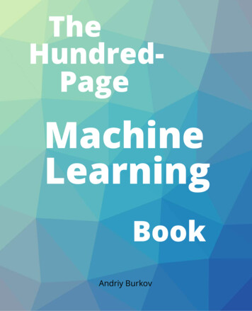
When the vector is on the left side of the matrix in the multiplication, then it has to betransposed before we multiply it by the matrix. The transpose of the vector x denoted as x makes a row vector out of a column vector. Let’s say,5 (1) 6xx (2) ,xthen,ËÈdefx x(1) , x(2) .The multiplication of the vector x by the matrix W is given by x W,ËÈ 5w(1,1) w(1,2) w(1,3) 6x W x(1) , x(2)w(2,1) w(2,2) w(2,3) def # (1,1) (1) wx w(2,1) x(2) , w(1,2) x(1) w(2,2) x(2) , w(1,3) x(1) w(2,3) x(2)As you can see, we can only multiply a vector by a matrix if the vector has the same numberof dimensions as the number of rows in the matrix.2.1.6FunctionsA function is a relation that associates each element x of a set X , the domain of the function,to a single element y of another set Y, the codomain of the function. A function usually has aname. If the function is called f , this relation is denoted y f (x) (read f of x), the elementx is the argument or input of the function, and y is the value of the function or the output.The symbol that is used for representing the input is the variable of the function (we oftensay that f is a function of the variable x).We say that f (x) has a local minimum at x c if f (x) Ø f (c) for every x in some openinterval around x c. An interval is a set of real numbers with the property that any numberthat lies between two numbers in the set is also included in the set. An open interval doesnot include its endpoints and is denoted using parentheses. For example, (0, 1) means greaterthan 0 and less than 1. The minimal value among all the local minima is called the globalminimum. See illustration in fig. 2.A vector function, denoted as y f (x) is a function that returns a vector y. It can have avector or a scalar argument.Andriy BurkovThe Hundred-Page Machine Learning Book - Draft6

642f(x) 0–2–4local minimumglobal minimum–6Figure 2: A local and a global minima of a function.2.1.7Max and Arg MaxGiven a set of values A {a1 , a2 , . . . , an }, the operator,max f (a)aœAreturns the highest value f (a) for all elements in the set A. On the other hand, the operator,arg maxf (a)aœAreturns the element of the set A that maximizes f (a).Sometimes, when the set is implicit or infinite, we can write maxa f (a) or arg maxf (a).aOperators min and arg min operate in a similar manner.2.1.8Assignment OperatorThe expression a Ω f (x) means that the variable a gets the new value: the result of f (x).We say that the variable a gets assigned a new value. Similarly, a Ω [a1 , a2 ] means that thetwo-dimensional vector a gets the value [a1 , a2 ].Andriy BurkovThe Hundred-Page Machine Learning Book - Draft7

2.1.9Derivative and GradientA derivative f Õ of a function f is a function or a value that describes how fast f grows (ordecreases). If the derivative is a constant value, like 5 or 3, then the function grows (ordecreases) constantly at any point x of its domain. If the derivative f Õ is a function, then thefunction f can grow at a different pace in different regions of its domain. If the derivative f Õis positive at some point x, then the function f grows at this point. If the derivative of f isnegative at some x, then the function decreases at this point. The derivative of zero at xmeans that the function’s slope at x is horizontal.The process of finding a derivative is called differentiation.Derivatives for basic functions are known. For example if f (x) x2 , then f Õ (x) 2x; iff (x) 2x then f Õ (x) 2; if f (x) 2 then f Õ (x) 0 (the derivative of any function f (x) c,where c is a constant value, is zero).If the function we want to differentiate is not basic, we can find its derivative using thechain rule. For example if F (x) f (g(x)), where f and g are some functions, then F Õ (x) f Õ (g(x))g Õ (x). For example if F (x) (5x 1)2 then g(x) 5x 1 and f (g(x)) (g(x))2 .By applying the chain rule, we find F Õ (x) 2(5x 1)g Õ (x) 2(5x 1)5 50x 10.Gradient is th

1.2.2 Unsupervised Learning In unsupervised learning, the dataset is a collection of unlabeled examples {x i}N i 1 Again, x is a feature vector, and the goal of an unsupervised learning algorithm is to create a model that takes a feature vector x as input and either transforms it into another vector or into a value that can be used to solve a practical problem. For example,