WIXLIB

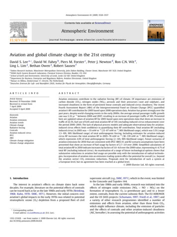
3522D.S. Lee et al. / Atmospheric Environment 43 (2009) 3520–3537(Forster et al., 2007a). Forster et al. (2007a) were unable to updatethe aviation forcings from Sausen et al. (2005) as fuel scalar datawere not available. Instead, the Sausen et al., 2005 RF values wereadopted as 2005 values, noting that they would likely to be within 10% of the actual 2005 value. IPCC’s Working Group three (WGIII),in conjunction with WGI, estimated that aviation represented 3% ofthe total anthropogenic RF in 2005, with an uncertainty rangebased on non-aviation forcings of 2–8% (Kahn-Ribeiro et al., 2007).The uncertainty range was set by the background anthropogenic RFrather than aviation effects, since Sausen et al. (2005) did not reportuncertainties for aviation RF components.Aviation passenger transport volume in terms of revenuepassenger kilometres (RPK) has continued to grow strongly at anaverage rate of 5.2% per annum over the period 1992–2005, despiteworld-changing events such as the first Gulf War, the World TradeCenter attack and outbreaks of Severe Acute Respiratory Syndrome(SARS) (Fig. 2). Aircraft manufacturers predict that the global civilfleet may nearly double from w20,500 aircraft in 2006–w40,500aircraft in 2026 (Airbus, 2007). Meanwhile, because of the stronggrowth rate of aviation and the resulting policy interests in mitigatingpotential future increases in emissions, climate research hascontinued since the IPCC (1999) report with the objective of reducingthe uncertainties of aviation’s non-CO2 effects, particularly the effectsof linear persistent contrails and AIC.Whereas it was concluded in the IPCC AR4 WGI report thataviation’s total RF in 2005 was within 10% of 2000 values becauseof slow growth in aviation fuel usage over the 2000–2005 period,recently available air traffic data from the International Civil Aviation Organization (ICAO) and kerosene fuel sales data from theInternational Energy Agency (IEA, 2007) indicate strong increasesin aviation activity and associated CO2 emissions over this period.These new data provided the initial motivation for the presentstudy. In the following we recalculate aviation 2005 RFs, assessuncertainties, provide new illustrative scenarios of 2050 aviationemissions and RFs, and examine potential mitigation opportunitiesafforded by technological improvements and policy-measures.2. Aviation radiative forcing in the IPCC FourthAssessment Report2.1. ContextThe IPCC AR4 WGI remit was to consider total anthropogenicand natural RFs for 2005, updating estimates for 2000 provided inthe Third Assessment Report (IPCC, 2001). The only RF componentsfor aviation considered explicitly were persistent linear contrailsand AIC, since other aviation contributions (e.g., CO2, O3/CH4, etc)were included in data and model calculations that treated theseother effects. The current state of knowledge of contrail and AIC RFsas assessed by IPCC AR4 and the use of metrics for aviation aresummarized in the following sections.2.2. Contrail radiative forcingFig. 2. (Top) Aviation fuel usage beginning in 1940 from Sausen and Schumann (2000)and extended with data from IEA (2007) and the IPCC Fa1 scenario of Henderson et al.(1999). The arrows indicate world events that potentially threatened global aviationuse: the oil crises of the 1970s, the Gulf war crisis in the early 1990s, the Asian financialcrisis in the late 1990s, the World Trade Center (WTO) attack in 2001 and the globalhealth crisis brought about by the severe acute respiratory syndrome (SARS). Alsoshown is the growth in air passenger traffic from 1970 to 2007 in billions (1012) ofrevenue passenger kilometres (RPK) (near right hand axis) (source: ICAO trafficstatistics from AirlineþTraffic.htmaccessed, 19 Sept. 2007) and the annual change in RPK (far right hand axis (Noteoffset zero)) (Bottom) Growth in CO2 emissions in Tg CO2 yr 1 for all anthropogenicactivities and from aviation fuel burn (left hand axis), and the fraction of totalanthropogenic CO2 emissions represented by aviation CO2 emissions (%) (right handaxis). Note 10 scaling of aviation CO2 emissions.The IPCC AR4 WGI estimate for contrail RF was based upon the workof Sausen et al. (2005) and references therein, which reassessed aviation for the year 2000 and provided a best estimate for persistent linearcontrails of 10 mW m 2. (A ‘best’ estimate is that estimate resultingfrom the IPCC assessment process and is usually associated with anuncertainty following IPCC nomenclature. See the Technical Summaryof IPCC AR4 WGI (p.23) (IPCC, 2007).) This value is approximatelya factor of three smaller than the contrail RF (33 mW m 2) that Sausenet al. (2005) obtained for 2000 by scaling the IPCC (1999) figures. Thesmaller estimate arises principally from recalculations of contrailcoverage and space and time dependent optical depths, which havealmost linear effects on the calculation of overall forcing (noting thatcontrail RF is the sum of two forcings, infrared and visible radiation,which have opposite signs). There remain significant uncertaintiesover contrail coverage and the optical depth of contrails (Schumann,2005; Forster et al., 2007a). The uncertainties in the contrail coveragearise from the lack of global observations of contrails and the poorlyknown extent of ice-supersaturation in the upper atmosphere. Icesupersaturation in the ambient atmosphere along an aircraft flighttrack is required for the formation of a persistent contrail. Ice-supersaturation is only measured locally with instrumental difficulty(e.g., Spichtinger et al., 2003) and estimated with significant uncertainty by global atmospheric models, although effort is beingcommitted to improving this (Tompkins et al., 2007). The uncertaintiesin the optical depth derive from uncertainties in the size distribution,number concentration, and shape of ice crystals.2.3. Aviation-induced cirrus cloud radiative forcingAviation-induced cirrus cloud cover is thought to arise from twodifferent mechanisms. The first (direct) mechanism is the formationof persistent linear contrails, which can spread through wind-shearto form cirrus-like cloud structures, sometimes called contrail-

D.S. Lee et al. / Atmospheric Environment 43 (2009) 3520–3537cirrus, that are eventually indistinguishable from natural cirrus. Alimited number of studies have provided estimates of trends in bothcontrails and AIC based on satellite data of cloudiness trends (Stordalet al., 2005; Stubenrauch and Schumann, 2005; Zerefos et al., 2003;Eleftheratos et al., 2007). The second (indirect) mechanism is theaccumulation in the atmosphere of particles emitted by aircraft atcruise altitudes, namely those containing black carbon, sulphate andorganic compounds (Kärcher et al., 2000) that may act as cloudcondensation nuclei. Here, the term aviation-induced cloudiness(AIC) is used to include both these mechanisms. Atmosphericmodels have shown that black carbon particles from aircraft couldeither increase or decrease the number density of ice crystals incirrus, depending on assumptions about the ice nucleation behaviour of the atmospheric (non-aircraft) aerosol in cirrus conditions(Hendricks et al., 2005). A change in the upper-tropospheric icenuclei abundance or nucleation efficiency can lead to changes incirrus cloud properties (Kärcher et al., 2007), including theirfrequency of formation and optical properties, which in turn changesthe RF contribution of cloudiness in the upper atmosphere.On the basis of correlation analyses, two studies (Zerefos et al.,2003; Stordal et al., 2005) attributed observed decadal trends incirrus cloud coverage to aviation from spreading linear contrails andtheir indirect effect. Both these studies used the InternationalSatellite Cloud Climatology Project (ISCCP) database and derivedcirrus cloud trends for Europe of 1–2% per decade over the last twodecades. A further study using different instrumental remotemeasurements provided support for such trends (Stubenrauch andSchumann, 2005) but not their magnitude, finding a trend approximately one order of magnitude smaller than those of Zerefos et al.(2003) and Stordal et al. (2005). Stordal et al. (2005) estimateda global RF for aviation cirrus with a mean value of 30 mW m 2 andan uncertainty range of 10–80 mW m 2, assuming similar opticalproperties to very thin cirrus. IPCC AR4 WGI adopted these valueswith the caveat that 30 mW m 2 does not constitute a ‘best estimate’in the same qualitative sense as other evaluated components ofanthropogenic climate forcing. Nonetheless, 30 mW m 2 is inreasonable agreement with the upper limit value of 1992 aviationcirrus forcing of 26 mW m 2 estimated by Minnis et al. (2004).2.4. Climate metrics for comparing emissions from aviationRadiative forcing is used here, as in previous studies, as thepreferred metric for quantifying the climate impact of aviation ata given point in time as a result of historical and current emissions.However, alternative metrics have been discussed for aviation andother sectors. There has been considerable debate on the subject ofemission equivalences, with Fuglestvedt et al. (2003, in press)providing comprehensive reviews. The usage of Global WarmingPotentials (GWPs) for aviation non-CO2 emissions was not considered specifically by WGI (Forster et al., 2007a), as did Prather et al.(1999), but were considered in the context of comparing GWPsfrom short-lived (e.g., O3) and long-lived species. Nonetheless,several of the studies reviewed by IPCC AR4 WGI (Forster et al.,2007a) considered O3 and CH4 changes from aviation NOx (Derwentet al., 2001; Stevenson et al., 2004; Wild et al., 2001). The difficultyin formulating a robust GWP for aviation NOx emissions wasrevealed in that whilst all three aforementioned studies consistently found positive AGWPs for the primary O3 increases andnegative AGWPs for CH4 and secondary O3 decreases, the balance ofthese terms was 100 and 130 in two of the studies, and 3 in thethird.In order to illustrate that aviation has significant climate forcings beyond the emission of long-lived greenhouse gases, Pratheret al. (1999) introduced the concept of the Radiative Forcing Index(RFI), which is the total aviation RF divided by the aviation CO2 RF.3523However, the RFI is not an emissions multiplier that can be used toaccount for aviation’s non-CO2 effects from future emissions. Thiswas confirmed by IPCC AR4 WGI (Forster et al., 2007a) in notingthat the RFI cannot account for the different atmospheric lifetimesof the different forcing agents involved, as previously explained byWit et al. (2005) and Forster et al. (2006, 2007b). However, nocriticism per se was made of the RFI metric when it is properlyunderstood and used. IPCC AR4 WGIII (Kahn-Ribeiro et al., 2007)clearly restated that ‘‘Aviation has a larger impact on radiativeforcing than that from its CO2 forcing alone’’.The difficulties involved in the inclusion of non-CO2 emissionsand effects into policy frameworks have been highlighted by IPCCAR4 WGIII (Kahn-Ribeiro et al., 2007) and others (e.g., Wit et al.,2005; Forster et al., 2006, 2007b). Thus far, a suitable metric to putnon-CO2 radiative effects on an equivalent emissions basis to CO2 forfuture aviation emissions has not been agreed upon because of thedifficulties of treating short-lived species and a long-lived speciessuch as CO2 in an equivalent manner. The metric used to compare theclimate impacts of long-lived GHG emissions under the KyotoProtocol is ‘equivalent CO2 emissions’ (i.e., emissions weighted witha 100-yr time horizon GWP). The equivalent-CO2 emission metric isa forward-looking metric, calculated for an emission pulse and,hence, suitable for comparing future emissions in a policy context.The RFI metric is primarily a backward looking metric because it canonly be used correctly with accumulated emissions of CO2 andtherefore is inherently unsuitable as an emissions-equivalencymetric for policy purposes. In terms of non-CO2 effects of aviation,the best current option may be to employ an additional policyinstrument(s) that would address these effects directly.3. Updating aviation radiative forcing in 20053.1. Aviation traffic and updated aviation fuel use for 2005Aviation traffic volume is reported, by convention, in RPK. Therehave been clear upward trends in both RPK and available seatkilometres (ASK, a measure of capacity cf. utilization) over decadaltimeframes but also over the period 2000–2005 (see Fig. 2), whichwould also imply an increase in fuel usage. As an accurate basis toupdate aviation RFs for 2005, recent kerosene fuel sales data foraviation operations were obtained from the IEA (IEA, 2007). Thesedata were used to extend and update a time-series of fuel usagebetween 1940 and 1995 (Sausen and Schumann, 2000) to 2005.Global civil air traffic declined in 2001 from 2000 levels in terms ofRPK, after which there was a small recovery in 2002, followed by anincrease of w2% from 2002 to 2003 (Fig. 2). From 2003 to 2004, therewas an unprecedented increase of 14% and a growth of 8% between2004 and 2005 such that overall, traffic increased by 22.5% (38%)between 2000 and 2005 (2007), although there are strong regionaldifferences (Airbus, 2007). Correspondingly, aviation fuel usageincreased by 8.4% in 2005 over that in 2000 according to IEA statistics.Various historical and projected aviation global CO2 inventoriesare shown in Fig. 3 for 1992–2050, along with IEA and other data. Itis clear from Fig. 3 that the IEA fuel sales data consistently indicatelarger CO2 emissions than implied by ‘bottom-up’ inventories. Thereare a number of reasons for this. Firstly, the inventories shown onlyestimate civil emissions; military emissions are much more difficultto estimate. Military emissions were calculated to be approximately11% of the total in 2002 (Eyers et al., 2005), cf. 18% as calculated byBoeing for 1992 (Henderson et al., 1999). Secondly, the IEA datainclude aviation gasoline, as used by small piston-engine aircraft,but this comprised only 2% of the total in 2000. Thirdly, theinventories are idealized in terms of missions in that great circledistances are often assumed and holding patterns are not included,nor the effect of winds. Finally, some inventories are based only on

3524D.S. Lee et al. / Atmospheric Environment 43 (2009) 3520–3537Fig. 3. Historical and present-day inventories, and future projections of civil aviationCO2 emissions from a variety of sources: AERO2K (Eyers et al., 2005); ANCAT/EC2(Gardner et al., 1998); CONSAVE (Berghof et al., 2005); FAST (Owen and Lee, 2006);IPCC (IPCC, 1999); NASA (Baughcum et al., 1996, 1998; Sutkus et al., 2001); SAGE (Kimet al., 2007). The open symbols indicate inventory analysis and the closed symbolsindicate projections. Also shown are the CO2 emissions implied by IEA fuel salesstatistics (IEA, 2007). The IEA data represent the total of civil and military usagebecause all kerosene sales are included. The Sausen and Schumann (2000) data arealso based on IEA. The solid (dashed) lines for FAST-A1 (B2) scenarios (evaluated withthe t1 technology option) and the IPCC Fa1 scenario also account for all fuel sales inorder to be consistent with the IEA values ending in 2005. In the figure legend, theFAST, CONSAVE, and IPCC symbols are shown in an order that matches the scenariolabels in the parentheses in each case. The IPCC Fa1 data for 1995–2006, the IEA dataand the Sausen and Schumann (2000) data are also shown in Fig. 2. Adapted fromFigure 5.6 of Kahn-Ribeiro et al. (2007).scheduled traffic, whereas others include estimates of non-scheduled traffic for the main air traffic regions. These various factorsconspire to systematically underestimate aviation CO2 emissions,an effect which has been known for some time but still remainsdifficult to reconcile. Thus, in RF calculations it is important to usethe total kerosene fuel sales data to calculate CO2 emissions and,thereby, reflect the total impact of all aviation activities.3.2. Modelling methodology for 2005 and 2050 aviationradiative forcing componentsThe RF for aviation CO2 is calculated explicitly, whereas otherRFs are calculated either directly or indirectly from fuel data frombase-year reference data from more complex models. The approachtaken to calculate aviation CO2 RF was to first calculate the CO2concentrations attributable to aviation using a carbon-cycle modeland then calculate its RF according to a simple function as recommended by the IPCC Third Assessment Report (Ramaswamy et al.,2001). The non-CO2 effects are scaled with fuel usage from reference values calculated with a suite of more complex models, butaccount for technological changes affecting emissions and othernon-linear effects (e.g., contrails) as described below.The model as described by Lim et al. (2007) is an extendedversion of a simplified climate model (SCM) for CO2 and NOxemissions effects on O3 (Sausen and Schumann, 2000) that is alsoused to account for other aviation emissions and effects. The nonCO2 effects were originally calibrated to the results from IPCC(1999) for 1992 and 2050, so that the model could be used withconfidence to project forwards in time (its main purpose is tocalculate temperature response, RF being an intermediate step).Having calibrated the evolution of aviation RFs over time with theIPCC (1999) results for 1992 and 2050, the model was recalibratedto a base-year of 2000 using the results of Sausen et al. (2005),which were derived from more complex models.This scaling approach to calculate future RFs is used here in theabsence of a complete and comprehensive set of RF calculationsfrom chemical transport models, contrail coverage models andradiative transfer codes. Such a comprehensive assessment is ofcourse preferable because of the sensitivities, for example, toregional effects and changes in climate parameters from nonaviation sources. The IPCC has accepted a similar approach (seeIPCC AR4 WGI, Meehl et al., 2007) for rapid low-cost computationsof future total RF and temperature response with the MAGICCmodel (Wigley, 2004) based on parameterizations that mimicensemble results of more complex models (Wigley et al., 2002).Moreover, IPCC (1999) used a similar approach to scale RFs fora range of 2050 aviation scenarios from a central set of resultscalculated for 2050 with more complex models. Ponater et al.(2006) used a similar approach to calculate scenarios for hypothetical future liquid hydrogen (LH2) powered fleet of aircraft, ashave Grewe and Stenke (2008) to project RFs from a supersonicaviation fleet. Similarly, Fuglestvedt et al. (2008) have examinedcontributions of the different transportation sectors to global RFand temperature response with an SCM.The CO2 RF was calculated using a complete time-series ofaviation fuel data as described above for the period 1940–2005.Emissions of CO2 from fuel burn were used to calculate CO2 atmospheric concentrations with the simple carbon-cycle model of Hasselmann et al. (1997). This model is based upon that of Maier-Reimerand Hasselmann (1987) and uses a 5-coefficient impulse responsefunction. Such convolution integral models have their limitationswhen compared with more complex carbon-cycle models but theyare considered to work well for small linear perturbations (Caldeiraet al., 2000), such as featured in this work. Background CO2 RFs weretaken from historical data and scenario projections from the MAGICCmodel v4.1 (Wigley, 2004), as published in the IPCC Third Assessment Report (IPCC, 2001). The RF contribution of aviation CO2 is thencalculated using the CO2 concentrations attributable to aviationusing the simple function recommended by Ramaswamy et al.(2001), which originates from Myhre et al. (1998).The RF reference value for O3 increases from NOx emissions isbased upon a calibration with the ensemble results from morecomplex chemical transport models (CTMs) and climate chemistrymodels (CCMs) that provided input to Sausen et al. (2005) for 2000,adjusted by a factor of 1.15 to agree with IEA fuel burn (Pratheret al., 1999). The O3 RFs are projected forward in time using valuesof the NOx emission index (EINOx, g NOx kg 1 fuel) from IPCC(1999). A linear relationship between O3 RF (or O3 burden) withincreases in aircraft NOx emissions at a global scale has been shownelsewhere to be a good approximation (e.g., IPCC, 1999 (Figure 4-3);Grewe et al., 1999; Rogers et al., 2002; Köhler et al., 2008; and alsofor shipping NOx perturbations, Eyring et al., 2007) over the rangeof NOx emissions used in these studies. Similarly, the referencevalue for the reduction in CH4 RF from NOx is calibrated to theresults of Sausen et al. (2005) for 2000 and scaled to the changes inO3 RF via EINOx projections. Thus far, potential non-linearities inthe atmospheric chemistry of NOx–O3 production (e.g., Jaeglé et al.,1998) have not been clearly exhibited in global models at largescales. Non-linearities have only clearly been manifested at scalessmaller than the globe (e.g. Rogers et al., 2002).Reference values for water vapour, SO4 and soot RFs werecalibrated to Sausen et al.’s (2005) values. Future values were scaledvia the respective emissio

Aviation and global climate change in the 21st century David S. Leea,*, David W. Faheyb, Piers M. Forsterc, Peter J. Newtond, Ron C.N. Wite, Ling L. Lima, Bethan Owena, Robert Sausenf aDalton Research Institute, Manchester Metropolitan University, John Dalton Building, Chester Street, Manchester M1 5GD, United Kingdom b NOAA Earth System Research Laboratory, Chemical Sciences Division, Boulder .