WIXLIB

Analog to Digital ConversionMeredith Matteson*Mentor: Aysha Shanta*Lenoir City High SchoolThe University of Tennessee KnoxvilleYoung Scholars Program, CURENT, EECS, UTK

About the AuthorsMeredith Marie MattesonMeredith Marie Matteson is an upcoming senior at Lenoir CityHigh School (LCHS) in Lenoir City, Tennessee. She is thePresident of the school’s Chapter of National Honor Society aswell as the Vice President of Mu Alpha Theta, theMathematics Honor Society. Meredith has a Varsity Track andField Letter and is in the Lenoir City High School top Choir Ensemble, The LCHS Singers. Shehas participated in the Newspaper Tower Competition and the Food Battery Competition at theannual Engineer’s Day at the University of Tennessee.Aysha Siddique ShantaAysha Siddique Shanta received the B.Sc. degree in electricalengineering from BRAC University, Dhaka,Bangladesh, in 2011,and is currently working towards the Ph.D. degree in computerengineering at the University of Tennessee,Knoxville, TN, USA.Her research interest include microelectrode design with carbonnanofibers and/or carbon nanospikes for electrochemical interfaces and she is also interested indevice modeling.i

AbstractThis project is about an analog to digital converter. The task is to write codes in MATLAB thatconvert an analog voice recording into a digital signal. The original recording has bothcontinuous time and continuous valued the final digital signal will have both discrete time anddiscrete value. The digital recording can be transmitted over the communication channel andprocessed digitally at the receiving end.ii

Table of ContentsIntroduction 1Literature Review 3Method 6Results 7Disscussion 9Conclusion 9Acknowledgements 10References 10Appendix 12iii

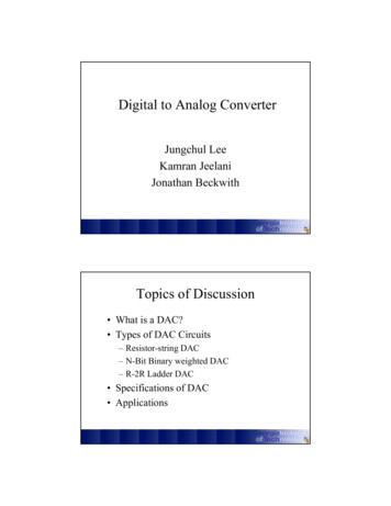
1I. INTRODUCTIONAnalog to Digital conversion (ADC) is a process that has very importantapplications in the modern world. Since most modern devices are digital, all analogsignals must be converted to digital signals. Digital devices are cheaper and moredependable. In addition, digital computers have the ability to manipulate, transmit, andprocess data in ways never thought possible before. Without this conversion, most of ourmodern technology would be unusable.Figure 1: Analog Signal [1]Figure 2: Digital Signal [2]Analog signals have continuous waves and an infinite number of data points asshown in Figure 1. Digital signals are made up of just enough of those points so that it ispossible to reconstruct the wave later at the receiving end. An example of a digital signalis shown in Figure 2. The process takes continuous data and makes it more efficient andpractical digital data. This digital data can then be transmitted from one place to anotherand processed digitally. The analog signal is inputted into an ADC to convert it into adigital input signal which is then inserted into a digital signal processor and changed intoa digital output signal. On the receiving end, it is reconstructed into an analog signal

2using an Digital to Analog converter [6]. Figure 3 represents a block diagram of thementioned process. .Figure 3: The process of analog to digital conversion and digital to analog reconstruction [6].A perfect example of this concept is the telephone. When calling someone, thevoice acts as the analog signal. It is converted into a digital signal using sampling,quantization, and coding, then transmitted and reconstructed on the other end of thetelephone line. This is why a person sounds different on the telephone than he or she doesin real life. Some other examples of an ADC are radio, cameras, video recorders,computers, and television. Digital signals are more practical due to the fewer amount ofdata points. The fewer data points allow the data to be transmitted and processed faster.In order to use any type of digital device, like a computer for example, the signal must bedigital. In the modern era, where computers are such a huge part of everyday life, analogto digital conversion is essential.

3Figure 4:Process of analog to digital conversion [6]Only the conversion from analog to digital signal has been completed in thisproject. This portion is made of three different steps: sampling, quantization, and coding.A more detailed description is shown in Figure 4 where each step must be completedbefore another can begin.II. LITERATURE REVIEWSampling is the process of changing the x axis quantities from continuously timedto discretely timed, as shown in figure 5. After sampling, the signal will have a definitenumber of points on the x axis instead of an infinite number of points.Figure 5: Process of Sampling [6]

4The process simplifies the x axis to a point where it is workable and reasonable.Having millions and millions of data points, when considerably less are needed, isinefficient and unnecessary.SamplingSampling should consist of enough data points so that the signal can bereconstructed accurately. According to the Nyquist Shannon sampling theorem, thismeans that the sampling frequency should be at least twice the actual wave frequency [6].For example, if the frequency of the wave is 100 hertz, the sampling frequency should beat least 200 hertz.Figure 6: Testing to the Nyquist Shannon Sampling TheoremIn some cases, it is better to sample at a rate three or four times that of the originalfrequency at a minimum, as described by Figure 6. Figure 12 in the Appendix is anexample of a sampling code. As a result of this concept, as frequency increases, samplingrate must also increase.

5Figure 7: The green line represents the actual wave; the points represent the sample.Notice that the reconstructed signal (red line) is not the same as the green line [5].If the sampling frequency is too small, the samples cannot be accuratelyinterpolated to get the actual signal at the receiving end. An example is shown in Figure7. The more data points you have the easier it will be to reconstruct the wave, but havingan unnecessary number of data points is counterproductive.QuantizationThe next step is quantization. The digital device can only communicate Y axisdata at specific levels. Figure 8 shows a graphic representation of the concept.

6Figure 8: The graphic describes the process of quantization [6].The more quantization levels there are, the more accurate and reconstructable theplot will be. Number of quantization levels are assigned using the number of bits. Thenumber of bits equation for determining the number of levels 2 . So if the number of bits is 8,8 the number of levels is 2 256. The range, from the maximum height to the minimumheight, will have 256 different levels. Most telephones use an 8 bit quantizer. Thisconverts the continuously valued y axis into a discretely valued y axis. Quantization hasone completely inevitable inaccuracy: quantization error. The fact that the computerabandons the original y axis values and assigns another number in the place of it is a lossof data. However, the only way to reduce the quantization error is to increase the numberof levels which in turn reduces the quantization step. Fewer quantization levels makes theprocess more efficient in transmission and processing but it will cause a largerquantization error. More quantization levels makes the process less efficient but thereconstruction of the data will be more accurate.CodingThe next step is coding. Coding is a very important step. It converts thequantization level indices into a binary sequence. Digital devices only understand lowlevel languages, like binary for example. As a result, the data points must be converted toa series of 1’s and 0’s for the computer to process it.The combination of all three steps converts a signal with continuous time andcontinuous value to one that has discrete time and discrete value.

7III. METHODThis project’s task was to sample, quantize, and code the conversion from ananalog signal to a digital signal. The original wave is the analog signal. In thisexperiment, the wave is a recording of the voice saying, “Hello. My name is Meredith.”The computer automatically changed the recording into a sampled digital signal sincecomputers cannot store analog signals. So, the first step of the process is resampling. Thisaudio signal was resampled at 8 KHz as this is the most common sampling rate amongtelephone communication.For this experiment, the computer utilized the function [y, Fs, bits] audioread(‘’) to read the audio signal. This built in function reads the audio file andoutputs the sample frequency, number of bits used in quantization, and the y values. Thenthe program utilized the function x resample(y, p, q) where p is a new smaller samplingrate, q is the sampling frequency and y will be recognized from the audioread equation.For quantization, a 4 bit quantizer was used. Seeing that number of levels number of bits 2 , so there will be 16 distinct levels. The results will show a large differencebetween the analog recording and digital recording. For a closer look at the program, seeFigure 13 in the Appendix.In this project the computer used the variable dec2bin() built in function. It converts the decimal values into binary numbers. The variable in the parentheses wasindex, the variable representing the indices of the quantization levels. This processconverted the level indices to binary.

8All of the method is computerized. For every step, a MATLAB code was written.More details about the final code can be found in Figure 14 in the Appendix.IV. RESULTSFigure 9: The original voice recording

9Figure 10: The sampled audio recordingFigure 11: Final digital signalV. DISCUSSIONThe graphic of the original audio signal, as shown Figure 9. It displays an infinitenumber of points. The sample signal, as shown in Figure 10 and displays the position ofeach of the thousands of samples. The final digital signal as shown in Figure 11. 16different levels of quantization can be seen.The difference between the original analog signal and the sampled digital signal issignificant. The only major difference between the two figures is that the sampledrecording displays each sample. Each sample is represented by an open circle. Every timeone puts any kind of continuous information into a computer, like an image or audio

10recording, the computer changes it from analog data into digital data. The samplingdefines the number of points and where they will occur.Figure 11 shows the digital signal where the previously sampled signal has beendivided into 16 different levels after using the 4 bit quantizer.VI. CONCLUSIONThe process that so much of modern life is based around is a mystery to manypeople. The MATLAB coding involved has been engineered for maximum efficiency.The process of sampling and quantization is supposed to simplify on the x and y axisesso that the data can be made digital. If the data was not transferred to digital, it would notbe able to be used with any digital technology: rendering it nearly useless in today’ssociety.VII. ACKNOWLEDGEMENTSI would like to thank, my mentor, Aysha Shanta for all of her valuable help duringthe process; the success of this project would not have been possible without her. I wouldlike to thank all of the CURENT faculty and staff members. I would like to thank myfellow Young Scholars for helping and supporting me throughout the various challengesassociated with this project.This work was supported in part by the Engineering Research CenterProgram of the National Science Foundation and the Department of Energyunder NSF Award Number EEC 1041877 and the CURENT Industry PartnershipProgram.