Transcription
PRESCRIPTIONSCOMPUTING PRESCRIPTIONSEditors: Isabel Beichl, isabel.beichl@nist.govJulian V. Noble, jvn@virginia.eduTHE FULL MONTEBy Julian V. NobleTHIS IS MY INAUGURAL COLUMN ASCOEDITOR OF COMPUTING PRESCRIP-TIONS, ALTHOUGH NOT MY FIRST APPEARANCEHERE (I WROTE A GUEST COLUMN A COUPLE OFyears ago1). So, a word of self-introduction is in order. Back inthe summer of 1960, while interning at Grumman Aircraft, Iwas assigned to learn the new language Fortran so that I couldprogram the company’s brand-new IBM 704. The rules of engagement were arcane—you wrote out the program on an official IBM programmer’s pad, submitted it to the keypunchoperators, and (if the Force were with you) got back a puncheddeck several days later. Then the fun began. Imagine debugging on a system with three-day job turnaround!Luckily, the next summer I got to program a Burroughs 220(in machine language) and an IBM 7090 (in Fortran II) in auniversity setting. We were actually allowed to touch the keypunch machines ourselves (or in the Burroughs’s case, the tapepunch). And—oh, joy!—the turnaround time was “only” 24hours! If you want some idea of what prehistoric computingwas like, read Fred Hoyle’s sci-fi novels, The Black Cloud(Lightyear, 1998) and Ossian’s Ride (Harper, 1959)—both havechapters whose “action” takes place in computer centers.The personal computer revolution began in the late1970s. I soon discovered that getting a program to run using interactive Basic on a desktop machine (such as the HP1000 or the NorthStar) was faster than on the big CDC6600 mainframe using Fortran. I even published a paper2whose computations were all done on a Sinclair ZX-81computer that ran overnight. It had a 4-MHz, 8-bit Z80chip, with an interpretive ROM Basic and 16 Kbytes ofRAM. It displayed 16 lines of 64 characters on a TV set andused a tape cassette player for storage. The personal computer was lots slower than a mainframe, but the answerscame out much faster—a paradox we all live with now.When I learned to program, computer science departments lay far in the future. For good or ill, I learned aboutprogramming through reading and practice. The upside is76that I acquired no linguistic prejudices along the way andfelt free to try anything. The downside is that I am still ignorant of things for which I did not have an immediate use.In 1985, mainly through force of circumstance, I began touse Forth for most programming, preferring it to the various dialects of Fortran and Basic that had served me untilthen. Although I still occasionally dabble in C and Lisp, Inow mostly use Forth and machine code.3,4 Although somemight consider this eccentric, to me it seems no more sothan the artificial machine language MIX that DonaldKnuth illustrates algorithms with.5 Hold the flames; program fragments in this column will always be pseudocode—I won’t slight anyone’s pet language.Forthcoming columns will explore prescriptions for anovel way to solve the Laplace equation, the right angle onkeeping orthogonal functions orthogonal, how to do algebra on a computer, finding roots of analytic functions, andso on. These ideas are not engraved in stone: I welcome suggestions and comments, up to and including guest columns,and I am sure my coeditor, Isabel Beichl, feels the same.Fun with uniform variatesThis column is about computing based on various forms ofrandom sampling, or Monte Carlo methods.6 To get the ballrolling, I illustrate with applications to evaluating integrals,and to simple simulation, before explaining the prescriptionthat inspired the column. (You can find the Forth code for allthe applications in this column, including the random-lookuptable objects, at www.phys.virginia.edu/classes/551.jvn.fall01under the link “Forth system and example programs” andsublink “Monte Carlo techniques.”)IntegrationOf course, regular CiSE readers already know how toevaluate integrals using Monte Carlo methods, but it can’thurt to begin with something simple. Monte Carlo integration works best for many dimensions (where it beats theheck out of repeatedly applying a quadrature rule), but forclarity, I work in only one dimension here. Consider Figure1’s graph of a continuous function. If you sprinkle pointsuniformly but randomly over the bounding rectangle (as a1521-9615/02/ 17.00 2002 IEEECOMPUTING IN SCIENCE & ENGINEERING
Figure 1. A typical function in its bounding box.yTarget areaxrainstorm would do), it seems intuitively clear that the ratioof the number n falling in the “target area” under the curveto the total number of points N approaches the ratio of thecorresponding areas as N increases:n N A A box .(1)N Because we know Abox, once we know n/N with sufficientprecision we’re done. This is sometimes called brute-forceMonte Carlo. The pseudocode might resemble Figure 2.If we apply this code to the function f(x) x(1 x) on theinterval (0, 1), within the bounding box 0 f 0.5, five runs(of 104 points each) produce 0.16840, 0.16465, 0.16705,0.16770, and 0.16525. Their average is 0.16661, and theirstandard deviation is 0.0016. The exact value is 1/6; that is,for this relatively smooth function, the standard error forone run is roughly 1 percent, which is just what we expect ina sample of 104.This brute-force approach is inefficient: it needs too manyrandom numbers. Because a function’s average value over aninterval is, by definition, its integral divided by the length ofthat interval, we have a dx f (x) (b a) f av .b(2)The trick is then to find an independent method for computing fav, which is where random sampling comes in. Themost direct approach picks N uniformvariates xk in (a, b) and definesdff av 1NNf (x k ) . k 1(3)This method is called straight samplingand has the advantage of requiring onlyone call per point to the built-in(pseudo) random-number generatorrather than two calls as in the bruteforce algorithm. In n dimensions, this isn versus n 1, so the advantage is not sogreat. (I assume your system contains areasonably good algorithm for generating random floating-point numbers uniformly distributed on the interval (0,1).By “reasonably good,” I mean it shouldMAY/JUNE 2002have a cycle length of at least 109 and should pass the usualtests of serial correlation.)A second strategy—and this leads toward this column’stheme—is to choose the points where they will matter most.Importance sampling6 takes variates from some nonuniformdistribution (see Equations 4 and 5) that mimics the function we want to integrate. If the known nonuniform distribution consists of step functions, we call the method stratified sampling. A related strategy uses antithetic variates, inwhich pairs of variates are anticorrelated with each other.Because 1 Var ( f f ′) 2 111(4) Var( f ) Var( f ′) Cov ( f , f ′) ,424where (since they are anticorrelated) the covariance of thepair ( f , f ′)df(Cov ( f , f ′) f f) ( f ′ f′) 0(5)is negative, the variance can be greatly reduced from straightsampling, meaning we need fewer points for a given probable precision. A physical example is the Buffon needle problem with perpendicular crossed needles, which I often assignas an exercise.Batting practiceSimple simulations often use uniform distributions to represent the odds for discrete events. For example, we mightwant to know the incidence of batting slumps in a regularSubroutine: inside?leave 1 if point (x,y) is inside the integration volume,0 if outsideMain: BruteForceNpoints 0Nunder 0BEGIN Npoints NmaxWHILE(initialize)(TRUE if inequality satisfied)(execute up to REPEAT if TRUE)(otherwise jump to DONE)randomly choose new pointNunder Nunder inside?Npoints Npoints 1REPEATDONEFigure 2. Pseudocode for brute-force Monte Carlo integration.77
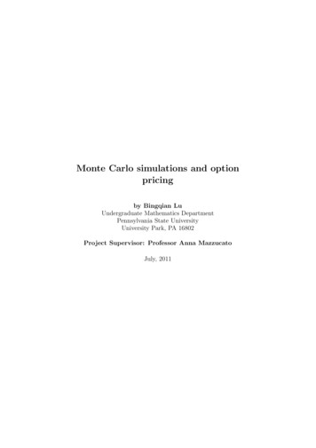
COMPUTING PRESCRIPTIONS\ Simulation of batting slumps\ data structures0.20e0 FVALUE p300 VALUE N10 VALUE mu0 VALUE hitless0 VALUE slumps\\\\\batting average# times @ bat/seasona “slump” is at least mu strikeoutscurrent # of hitless @ bats# slumps this seasonNormal variates\ programfunction: hit?Rand p\ it’s a hit if Rand p\ inequalities leave a flagfunction: slump?hitless mu\ it’s a slump if hitless musubroutine: end slumpslump?What if you want to simulate aprocess for which the events are notrepresentable by uniform variates inthe interval (0, 1)? Because feet followthe normal (that is, Gaussian) distribution, a shoe manufacturer’s statistician would sample normally distributed random variables. Here are twosatisfactory algorithms.First, choose 12 independent uniform variates 0 ξk 1 and define\ was there a slump going?IF slumps slumps 1 ENDIFhitless 0\ reset—slump is endedsubroutine: at batN 0 DO hit?IFend slumpELSEhitless hitless 1ENDIFLOOP12x It is easy to see that x has mean 0 andvariance 1. The Central Limit theorem, which says that a sum of independent random variables is (to a goodapproximation) normally distributed,assures that x is a normal variate. InFortran-ish pseudocode,Figure 3. Monte Carlo simulation of batting slumps.10 stats10 trials of 300 at bats, giving 55slumps. ok10 stats10 trials of 300 at bats, giving 66slumps. okand so forth. A 0.200 hitter has approximately 6 0.8 slumpsper season, whereas a 0.350 hitter would only experience1.2 0.2. The moral seems to be that he who bats betterslumps less—managers take note! Theory predicts roughly(N µ)p(1 p)µ per N at bats. For N 300, µ 10, andp 0.2, the formula predicts 6.2 slumps.78(6)kMain: stats (#cases --)LOCALS #cases hitless 0\ initializeslumps 0#cases 0 DO at batLOOP#cases report\ output resultsbaseball season of 162 games. If a batting slump is definedas µ at bats without a hit, then if a player bats, say, 300 timesper season, how many slumps will he experience?To simulate this Markov process, we assume the player’sbatting average p is his fixed probability of a hit each time atbat. With each event independent, our program resemblesFigure 3. Typical runs for a 0.200 hitter give 1 ξk 6 .FUNCTION normalsum -6e0DO 1, I 1,12 (add 12 PRNs)sum sum Rand1 CONTINUEnormal sumThe Box-Muller algorithm7 is a useful alternative whosespeed is comparable on some machines. Because dx dy e ( x2 y2)2 dθ dρe ρ22,(7)if we choose θ uniformly distributed on [0, 2π] and2η e ρ 2 ,(8)uniformly distributed on (0,1), we generate two independent, normally distributed random variables:a 2ln η cos θ(9a)b 2ln η sin θ .(9b)The algorithm in this form requires three transcendentalfunctions (log, sin, and cos) and a square root to generatetwo normal variates, so it is a bit expensive compared withgenerating a dozen uniform variates. George Box andMervin Muller discovered a useful trick, based on an earlierCOMPUTING IN SCIENCE & ENGINEERING
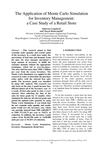
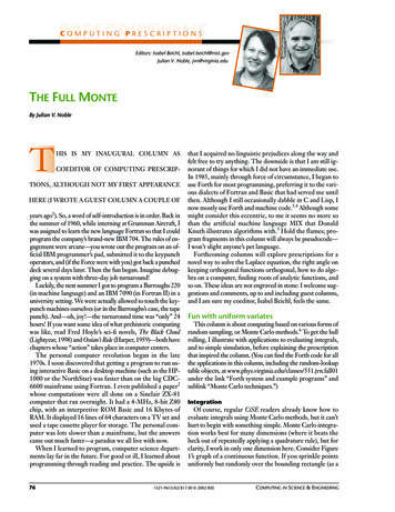
Figure 4. The Box-Muller algorithm for normal variates.Subroutine: Box MullerIFLastCall TRUETHENreturn yset LastCall FALSEELSEBEGIN(loop until u 1)x -1 2 * Randy -1 2 * Randu x 2 y 2u 1 UNTIL (end of loop)u sqrt (-(2 * ln (u)) / u)x x * uy y * ureturn xset LastCall TRUEENDIFgood. Figure 5 shows a sample of what the algorithmproduces.Arbitrary variatesMany physical processes are represented neither by uniform nor by normal variates. So, what do we do then? Tosample from an arbitrary probability distribution, if the cumulative distributions for two sets of random variables areidea of John von Neumann’s:8 if x and y are independent uniform variates on the interval (1, 1), the combination[](u x y θ 1 x y2222)P (x) xp(x ′)dx ′(12a)Q(ξ) ξξp(ξ ′)dξ ′(12b)(10)is uniformly distributed over the interval (0,1). Therefore aand b defined bya x 2ln u u(11a)b y 2ln u u(11b)are independent normally distributed random numbers onthe interval ( , ), each with mean 0 and variance σ 2 1.Now we only need compute approximately 2.5 uniform random numbers (strictly, 8/π), one transcendental function,and one square root per two normal variates. Figure 4 showsthe pseudocode. Because x and y are independent, we compute two variates every other time the subroutine is called.We then return one and save the other (to return on alternate calls). The global flag variable LastCall keeps track ofwhere we are. On the average, we compute an unsatisfactoryrandom pair (lying outside the circle) a tad less than 25 percent (that is, 1 π/4) of the time, so the efficiency is prettyxminminand if we set P(x(ξ)) Q(ξ), then our problem is to find thefunction x(ξ). Pretend this is a known function, and differentiate both sides with respect to ξ: we get an ordinary differential equation,p(x ) dx q(ξ) ,dξ(13)that we could, in principle, integrate numerically. However,because the distribution at our disposal is typically the uniform one, the easiest thing to do is solve the transcendentalequationx(ξ x)minp(x ′)dx ′ ξ(14)for a uniform variate ξ. Figure 6 is the result of inverting thisequation, for the case p(x) xe 12Figure 5. A histogram of 500 normal variates from theBox-Muller algorithm.MAY/JUNE 20023012345678910Figure 6. A histogram of 1,000 variates from xe x usinginversion.79
COMPUTING PRESCRIPTIONS45.040.536.031.527.0technical term is “good enough for government work”). Depending on the available storage, we could sufficiently finegrain the histogram so as not to incur any loss of “physicalsignificance.” To construct such a representation, it isenough to create a table of N variates Xk by solving theequation22.518.013.59.04.50.0012345678910 xXkminFigure 7. A histogram of 1,000 variates from xe x usingrejection.Alternatively, we could sample the distribution p(x) usingthe rejection method:8 choose a random variable η from auniform distribution on (0, 1), and choose a value of x in thedomain of p(x) by appropriate scaling. Then, ifηpmax p(x),(15)we keep the point x; otherwise, we reject it. (This resemblesthe Box-Muller algorithm, and works for the same reason.)Figure 7 shows a histogram of 1,000 such variates from thesame distribution xe x.Manifestly, the inverse and rejection methods both generate acceptable distributions. To illustrate, Figure 8 is outputfrom a simulation of the Young two-slit experiment, showinghow a diffraction pattern builds up from individual photons.(I have done versions using either inversion or rejection—there seems littledifference in execution speed, althoughI had expected rejection to be significantly faster.) The probability distribution, in the direction perpendicular tothe slits, is proportional to cos2x. Thescreen shot contains 500 “photons.”p(x ′)dx ′ k, k 0, , N 1.N(16)Now, in what sense does such a table represent the desiredrandom process? If we sample it by generating random indices into the table, the variates we randomly sample will approximate variates drawn from the original distribution. Forexample, Figure 10 shows a histogram of 1,000 samples fromthe distribution p(x) xe x, retrieved from a table with only64 entries. The results are quite acceptable. And, of course,by doing it this way, we only have to generate one randominteger and no expensive functions whenever we want a random variate. Although the table used in Figure 10 has only64 26 entries, my random-number generator has a cyclelength of 231, so there are 225 3 107 possible ways for itto traverse the table (a lot fewer than the 64! 1089 possibleorderings of a 64-entry table but big enough for most purposes). Even if you want a more fine-grained table, it getsconstructed once, so the time consumed in solving the transcendental equation N times is unimportant.Random objectsAll the preceding was preamble: Iam now about to Prescribe. In a largesimulation, both the rejection and inverse algorithms are generally far tooslow. The solution is a random-lookuptable. This is equivalent to replacingthe actual distribution function p(x)with a step-function approximation toit, as Figure 9 shows.For many simulations, a histogramrepresentation of the nonuniform distribution is perfectly adequate (the80Figure 8. A screen shot of 500 “photons” passing through parallel slits.COMPUTING IN SCIENCE & ENGINEERING
012345678910–1012345678910Figure 9. A histogram approximation of p(x) xe x by itsaverage over equal intervals.Figure 10. A histogram of 1,000 variates from xe x using a 64entry random-lookup table.In Fortran or C, we must construct each random-lookuptable by hand, define an array to hold the table, and then define a function that uses that array. The array must be filledbefore the program proper is executed by another subroutine written to do that. By contrast, extensible languagessuch as Lisp and Forth, as well as object-oriented ones suchas C , SmallTalk, or Forth, provide tools for defining constructors that can generate as many (independent) namedlookup tables as we like. Each such table becomes an object—data packaged with code that automatically performsthe table lookup—including, if desired, its own randomnumber generator. By using different generators (or different seeds) for different tables (even if they represent thesame distributions), we can eliminate problems arising fromserial correlations (that is, a given uniform generator mightnot be random enough, even though it passes standard tests).References1. J.V. Noble, “Gauss-Legendre Principal Value Integration,” Computing inScience & Eng. vol. 2, no. 1, Jan. 2000, pp. 92–95.2. J.V. Noble, “Missing Longitudinal Strength Cannot Reappear at VeryHigh Energy,” Phys. Rev. C, vol. 27, no. 1, Jan. 1983, pp. 423–425.3. J.V. Noble, Scientific Forth: A Modern Language for Scientific Computing,Mechum Banks Publishing, Ivy, Va., 1992.4. J.V. Noble, “Technology News & Reviews: Adventures in the Forth Dimension,” Computing in Science & Eng., vol. 2, no. 5, Sept. 2000, pp.6–10.5. D.E. Knuth, The Art of Computer Programming, 3rd ed., vol. 1, AddisonWesley, Boston, 1997, p. 124.6. J.M. Hammersley and D.C. Handscomb, Monte Carlo Methods, Methuen& Co., London, 1964, p. 57.7. G.E.P. Box and M.E. Muller, Annals Math. Statistics, vol. 29, 1958, p.610.8. J. Von Neumann, National Bureau of Standards Applied Mathematics Series, vol. 12, 1951, p. 36.9. I. Beichl and F. Sullivan, “Pay Me Now or Pay Me Later,” Computing inScience & Eng., vol. 1, no. 4, July/Aug. 1999, pp. 59–62.Ifirst used this technique to simulate the passage of highenergy particles through large atomic nuclei. An incidentparticle interacts differently with neutrons and protons; theyin turn have their own momentum and spin distributions.What happens depends not only on the initial conditions butalso on the branching probabilities for the various types ofreactions that can occur. It gets very complex very quickly,and you’d have to repeat the “experiment” millions of timesto obtain adequate statistics. It was helpful to be able to create named lookup objects for each different statistical distribution, which, when invoked, would return the appropriate sample variate. I hope you find this trick equally helpful.Happy computing!As an afterword, I should note that at least two earlier Computing Prescriptions have discussed methods for generatingvariates from nonuniform distributions.9,10 Of particular relevance is Alastair Walker’s “alias” method,11,12 explained byDonald Knuth13 and featured in Isabel Beichl and Francis Sullivan’s column,9 because it uses a precomputed lookup table.MAY/JUNE 200210. W.J. Thompson, “Poisson Distributions,” Computing in Science & Eng.,vol. 3, no. 3, May/June 2001, pp. 79–82.11. A.J. Walker, “New Fast Method for Generating Discrete Random Numbers with Arbitrary Frequency Distributions,” Electronics Letters, vol. 10,no. 8, 1974, pp. 127–128.12. A.J. Walker, “An Efficient Method for Generating Discrete Random Variables with General Distributions,” ACM Trans. Math. Software, vol. 3, no.3, Sept. 1977, pp. 253–256.13. D.E. Knuth, The Art of Computer Programming, 2nd ed., Addison-Wesley,Boston, 1981, vol. 2, pp. 115–119.Julian Noble is a professor of physics at the University of Virginia’s Department of Physics. His interests are eclectic, both in and out of physics.His philosophy of teaching computational methods is “no black boxes.”He received his BS in physics from Caltech and his MA and PhD in physicsfrom Princeton. He is a member of the American Physical Society, theACM, and Sigma Xi. Contact him at the Dept. of Physics, Univ. of Virginia, PO Box 400714, Charlottesville, VA 22904-4714; jvn@virginia.edu.81
The rules of en-gagement were arcane—you wrote out the program on an of- . read Fred Hoyle's sci-finovels, The Black Cloud (Lightyear, 1998) and Ossian's Ride(Harper, 1959) . baseball season of 162 games. If a batting slump is defined as µat bats without a hit, then if a player bats, say, 300 1 CONTINUEtimes .