Transcription
April 12, 2013Comments WelcomeMomentum CrashesKent Daniel and Tobias Moskowitz - Abstract -Across numerous asset classes, momentum strategies have historically generatedhigh returns, high Sharpe ratios, and strong positive alphas relative to standardasset pricing models. However, the returns to momentum strategies are skewed:they experience infrequent but strong and persistent strings of negative returns.These momentum “crashes” are forecastable: they occur following market declines,when market volatility is high, and contemporaneous with market “rebounds.”The data suggest that low ex-ante expected returns in crash periods result from aa conditionally high premium attached to the option-like payoffs of the past-loserportfolios. We show that an implementable dynamic strategy based on our analysis generate a Sharpe-ratio approximately double that of the static momentumstrategy. Finally, we show that the anomalous returns to momentum strategy arecorrelated with but not explained by volatility risk. Columbia Business School and Booth School of Business, University of Chicago, respectively. Contact information: kd2371@columbia.edu and Tobias.Moskowitz@chicagobooth.edu. For helpful comments and discussions, we thank Pierre Collin-Dufresne, Gur Huberman, Mike Johannes, Tano Santos, Paul Tetlock, SheridanTitman, Narasimhan Jegadeesh, Will Goetzmann, and participants of the NBER Asset Pricing Summer Institute, the Quantitative Trading & Asset Management Conference at Columbia, the 5-Star Conference at NYU,and seminars at Columbia, Rutgers, University of Texas, Austin, USC, Yale, Aalto, BI Norwegian BusinessSchool, Copenhagen Business School, the Q group and Kepos Capital and SAC.
1IntroductionA momentum strategy is a bet that past returns will predict future returns. Consistent withthis, a long-short momentum strategy is typically implemented by buying past winners andtaking short positions in past losers.Momentum appears pervasive: the academic finance literature has documented the efficacyof momentum strategies in numerous asset classes, from equities to bonds, from currenciesto commodities to exchange-traded futures.1 Momentum is strong: in US equities, wherethis investigation is focused, we see an average annualized return difference between the topand bottom momentum deciles of 16.5%/year, and an annualized Sharpe ratio of 0.82 (PostWWII, through 2008).2 This strategy’s beta over this period was -0.125, and it’s correlationwith the Fama and French (1992) value factor was strongly negative.3 Momentum is a strategyemployed by numerous quantitative investors within multiple asset classes and even by mutualfunds managers in general.4However, the strong positive returns of momentum strategies are punctuated with strongreversals, or “crashes.” Like the returns to the carry trade in currencies, momentum returnsare negatively skewed, and the crashes can be pronounced and persistent.5 In our 1927-2010sample, the two worst months for the aforementioned momentum strategy are consecutive:July and August of 1932. Over this short period, the past-loser decile portfolio returned236%, while the past-winner decile saw a gain of only 30%. In a more recent crash, over thethree-month period from March-May of 2009, the past-loser decile rose by 156%, while thedecile of past winners portfolio gained only 6.5%.1A fuller discussion of this literature is given in Section 2Section 3 gives a detailed description of the construction of these value-weighted momentum portfolios,and summary statistics on their performance.3Not surprisingly, momentum returns are not priced by either the CAPM or the Fama and French (1993)three-factor model (see Fama and French (1996)). A Fama and French (1993) model augmented with amomentum factor, as proposed by Carhart (1997) is necessary to explain the momentum return. Also notethat Asness, Moskowitz, and Pedersen (2008) argue that a three factor model (based on a market factor,and a value and momentum factor) is successful in pricing value and momentum anomalies in cross-sectionalequities, country equities, commodities and currencies.4Jegadeesh and Titman (1993) motivate their investigation of momentum with the observation that “. . . amajority of the mutual funds examined by Grinblatt and Titman (1989, 1993) show a tendency to buy stocksthat have increased in price over the previous quarter.”5See Brunnermeier, Nagel, and Pedersen (2008), and others for evidence on the skewness of carry tradereturns.21
We investigate the predictability of these momentum crashes. At the start of each of thetwo crashes discussed above (July/August of 1932 and March-May of 2009), the broad USequity market was down significantly from earlier highs. Market volatility was high. Also,importantly, the market as a whole rebounded significantly in these momentum crash months.This is consistent with the general behavior of momentum crashes: they tend to occur intimes of market stress, specifically when the market has fallen and when ex-ante measures ofvolatility are high. They also occur when contemporaneous market returns are high. Notethat our result here is consistent with that of Cooper, Gutierrez, and Hameed (2004) andStivers and Sun (2010), who find, respectively, that the momentum premium falls to zerowhen the past three-year market returns has been negative and that the momentum premiumis low when market volatility is high.These patterns are suggestive of the possibility that the changing beta of the momentumportfolio may partly be driving the momentum crashes. The time variation in betas of return sorted portfolios was first documented by Kothari and Shanken (1992). Grundy andMartin (2001) apply Kothari & Shanken’s insights specifically to price momentum strategies.Intuitively, the result is straightforward, if not often appreciated: when the market has fallensignificantly over the momentum formation period – in our case from 12 months ago to 1month ago – there is a good chance that the firms that fell in tandem with the market wereand are high beta firms, and those that performed the best were low beta firms. Thus, following market declines the momentum portfolio is likely to be long low-beta stocks (the pastwinners), and short high-beta stocks (the past losers).We verify empirically that there is dramatic time variation in the betas of momentum portfolios. Using beta estimates based on daily momentum decile returns we find that, followingmajor market declines, betas for the past-loser decile rise above 3 , and fall below 0.5 for pastwinners.However, GM further argue that performance of the momentum portfolio is dramaticallyimproved — particularly in the pre-WWII era, by dynamically hedging the market and sizerisk in the portfolio. While we replicate their results with a similar methodology, overall ourempirical results do not support GM’s conclusion. The reason for this is that, when GM createtheir hedged momentum portfolio, they calculate their hedging coefficients based on forward-2
looking measured betas.6 Therefore, their hedged portfolio returns are not an implementablestrategy.GM’s procedure, while not technically valid, should not bias their estimated performance iftheir forward-looking betas are uncorrelated with future market returns. However we showthat this correlation is present, is strong, and does bias GM’s results.7The source of the bias is a striking correlation of the loser-portfolio beta with the return on themarket. In a bear market, we show that the up- and down-market betas differ substantially forthe momentum portfolio. Using Henriksson and Merton (1981) specification, we calculate upand down-betas for the momentum portfolios.8 We show that, in a bear market, momentumportfolio up-market beta is more than double its down-market beta ( 1.47 versus 0.66), andthat this difference is highly statistically significant (t 5.1). Outside of bear markets, thereis no statistically significant difference.More detailed analysis shows that most of the up- versus down-beta asymmetry in bear marketis driven by the decile of past-losers: for this portfolio the up- and down betas differ by 0.6,while for the past-winner decile the difference is -0.2.Our examination of momentum crashes outside the US and other asset classes reveals similarpatterns. In Section 7, we show that the same option-like behavior is present for cross-sectionalequity momentum strategies in Europe, Japan, the UK, and for a global momentum strategy.In addition the optionality is a feature of commodity- and currency-momentum strategies.There are several possible explanations for this option-like behavior. For the equity momentumstrategies, one possibility is that the optionality arises because, for a firm with debt in itscapital structure, a share of common stock is a call option on the underlying firm value (Merton1990). Particularly in the distressed periods where this option-like behavior is manifested, theunderlying firm values in the past loser portfolio have generally suffered severe losses, and aretherefore potentially much closer to a level where the option convexity would be strong. Thepast winners, in contrast, would not have suffered the same losses, and would still be in-the6At the time GM undertook their study, only monthly CRSP data was available in the pre-1972 sampleperiod. They therefore used a five-month forward-looking regression to determine the hedging coefficients.7A recent paper by Boguth, Carlson, Fisher, and Simutin (2010) provides a critique Grundy and Martin(2001) and a set of other papers which “overcondition.” in a similar way.8Following Henriksson and Merton (1981), the up-beta is defined as the market-beta conditional on thecontemporaneous market return being positive, and the down-beta is the market beta conditional on thecontemporaneous market return being negative.3
money. This hypothesis, however, does not seem plausible for the commodity and currencystrategies, which also exhibit strong option-like behavior. In the conclusion we briefly discussa behaviorally motivated explanation for this phenomenon, but a fuller understanding is anarea for future research.One question that naturally arises given this finding is whether the time variation in themomentum premium we document here is related to time-varying exposure to volatility risk.We investigate this question in Section 6.2. We show that, in volatile bear markets, wml has ahigh negative exposure to a factor based on the return to an S&P 500 variance swap: that is,moemntum is effectively short volatility in panic periods. However, the loading on variancerisk does not appear to be responsible for the changing momentum premium in these periods.The layout of the paper is as follows: In Section 2 we review the literature we build upon inour analysis. Section 3 describes the data and portfolio construction. Section 4 documentsthe empirical analysis for momentum strategies in US equities. In Section 5 we examine theperformance of a optimal dynamic strategy based on our findings here. We also perform subsample analysis as a robustness check, and show that the strong performance of the dynamicstrategy relative to the base strategy is present in each approximately quarter-century subsample. In Section 6 we investigate whether the anomalous performance of the momentumstrategy can be explained by dynamic loadings on size, value or volatility factors. Section 7performs similar analysis on momentum strategies in international equities and in other assetclasses. Section 8 speculates about the sources of the premia we observe, discusses areas forfuture research, and concludes.2Literature ReviewA momentum strategy purchases assets with strong recent performance, and sells assets withpoor recent performance. The performance of momentum strategies in U.S. common stockreturns is documented in Jegadeesh and Titman (1993, JT). JT examine portfolios formedby sorting on past returns. For a portfolio formation date of t, their portfolios are formedon the basis of returns from t τ months up to t 1 month.9 JT examine strategies for τbetween 3 to 12 months, and hold these portfolios between 3 and 12 months. Their data is9The motivation for skipping the last month prior to portfolio formation is the presence of the short-termreversal effect as documented by Jegadeesh (1990).4
from 1965-1989. For all horizons, the top-minus-bottom decile spread in portfolio returns isstatistically strong. However, JT also note the poor performance of momentum strategies inpre-WWII US data.Jegadeesh and Titman (2001) note the continuing efficacy of the momentum portfolios incommon stock returns from the time of the publication of their original paper.2.1Momentum in Other Asset ClassesStrong and persistent momentum effects are also present outside of the US equity market. Rouwenhorst (1998) finds evidence of momentum in equities in developed markets, andRouwenhorst (1999) documents momentum in emerging markets. Asness, Liew, and Stevens(1997) demonstrates positive abnormal returns to a country timing strategy which buys acountry index portfolio when that country has experienced strong recent performance, andsells the indices of countries with poor recent performance. Momentum is also present outsideof equities: Okunev and White (2003) find momentum in currencies; Erb and Harvey (2006)in commodities; Moskowitz, Ooi, and Pedersen (2012) in exchange traded futures contracts;and Asness, Moskowitz, and Pedersen (2008) in bonds. Asness, Moskowitz, and Pedersen(2008) also integrate the evidence on within-country cross-sectional equity, country-equity,country-bond, currency, and commodity value and momentum strategies.Among common stocks, there is evidence that momentum strategies perform well for industrystrategies, and for strategies that are based on the firm specific component of returns (seeMoskowitz and Grinblatt (1999), Grundy and Martin (2001).)2.2Sources of MomentumThe underlying mechanism responsible for momentum is as yet unknown. By virtue of thehigh Sharpe-ratios associated with the momentum effect, these return patterns are difficult toexplain within the standard rational-expectations asset pricing framework. Following Hansenand Jagannathan (1991), In a friction-less framework the high Sharpe-ratio associated withzero-investment momentum portfolios implies high variability of marginal utility across statesof nature. Moreover, the lack of correlation of momentum portfolio returns with standardproxy variables for macroeconomic risk (e.g., consumption growth) sharpens the puzzle still5
further (see, e.g., Daniel and Titman (2012))A number of behavioral theories of price formation proport to yield momentum as an implication. Daniel, Hirshleifer and Subrahmanyam (1998, 2001) propose a model in whichmomentum arises as a result of the overconfidence of agents; Barberis, Shleifer, and Vishny(1998) argue that a combination of representativeness; Hong and Stein (1999) model twoclasses of agents who process information in different ways; Grinblatt and Han (2005) arguethat agents are subject to a disposition effect, and as a result are averse to recognizing losses,and are too quick to sell past winners.10 George and Hwang (2004) point to a related anomaly– the 52-week high – and argue that it is a result of anchoring on past prices.2.3Time Variation in Momentum Risk and ReturnKothari and Shanken (1992) argue that, by their nature, past-return sorted portfolios willhave significant time-varying exposure to systematic factors. Because momentum strategiesare bets on past winners, they will have positive loadings on factors which have had a positiverealization over the formation period of the momentum strategy. For example, if the marketwent up over the last 12 months, a 12-month momentum strategy will be long high-beta stocksand short low-beta stocks, and will therefore have a high market beta.Grundy and Martin (2001) note the time variation in the betas of momentum strategy, andfurther argue that the Fama and French (1993) market, value and size factors do not explainthe returns to a momentum strategy. In fact, they show that hedging out a momentum strategy’s dynamic exposure to size and value factors dramatically reduces the strategy’s returnvolatility, increases the Sharpe ratio, and eliminates the momentum strategy’s historicallypoor performance in January, and it’s poor record in the pre-WWII period. However, as wediscuss in Section 4.4, their hedged portfolio is constructed based on forward-looking betas,and is therefore not an implementable strategy. In this paper, we show that this results in astrong bias in estimated returns, and that a hedging strategy based on ex-ante betas does notexhibit the performance improvement noted in GM.Cooper, Gutierrez, and Hameed (2004) examine the time variation of average returns to USequity momentum strategies. They define UP and DOWN market states based on the lagged10Frazzini (2006) examines the presence of the disposition effect on the part of mutual funds.6
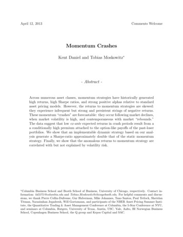
three-year return of the market. They find that in UP states, the historical mean return to aequal-weighted momentum strategy is 0.93%/month. In contrast in DOWN states the meanreturn has been -0.37%/month. They find similar results, controlling for market, size & valuebased on the unconditional loadings of the momentum portfolios on these factors.11Finally, the result that the betas of winner-minus-loser portfolios are non-linearly related tocontemporaneous market returns has also been documented elsewhere. In particular Rouwenhorst (1998), documents this feature for non-US momentum strategies.12 However, Chan(1988) and DeBondt and Thaler (1987) earlier document this non-linearity for longer-termwinner/loser portfolios is non-linearly to the market return, though DeBondt and Thaler dotheir analysis on the returns of longer-term winners and losers as opposed to the shorter-termwinners and losers we examine here. Boguth, Carlson, Fisher, and Simutin (2010), building onthe results of Jagannathan and Korajczyk (1986), note that the interpretation of the measuresof abnormal performance (i.e., the alphas) in Chan (1988), Grundy and Martin (2001) andRouwenhorst (1998) are problematic.3Data and Portfolio ConstructionOur principal data source is CRSP. Using CRSP data, we construct monthly and daily momentum decile portfolios. Both sets of portfolios are rebalanced only at the end of each month.The universe start with all firms listed on NYSE, AMEX or NASDAQ as of the formationdate. We utilize only the returns of common shares (with CRSP share-code of 10 or 11).We require that the firm have a valid share price and a valid number of shares as of theformation date, and that there be a minimum of 8 valid monthly returns over the 11 monthformation period. Following convention and CRSP availability, all prices are closing prices,and all returns are from close to close.Figure 1 illustrates the portfolio formation process used in determining the momentum portfolios returns for the one month holding period of May 2009. To form the portfolios, we beginby calculating ranking period returns for all firms. The ranking period returns are the cumulative returns from close of the last trading day of April 2008 through the last trading day ofMarch 2009. Note that, consistent with the literature, there is a one month gap between the11Cooper, Gutierrez, and Hameed (2004) do not calculate conditional risk measures, e.g. using the instruments proposed by Grundy and Martin (2001).12See, Table V, p. 279.7
Figure 1: Momentum Portfolio ConstructionThis figure illustrates the formation of the momentum decile portfolios. As of close of thefinal trading day of each month, firms are ranked on their cumulative return from 12 monthsbefore to one month before the formation date.t-12t-2May '08MarchRanking Period(11 months)Formation Datet(April)May '09HoldingPeriod(1 mo.)end of the ranking period and the start of the holding period.All firms meeting the data requirements are placed into one of ten decile portfolios on thebasis of their cumulative returns over the ranking period. However, the portfolio breakpointsare based on NYSE firms only. That is, the breakpoints are set so that there are an equalnumber of NYSE firms in each of the 10 portfolios.13 The firms with the highest ranking periodreturns go into portfolio 10 – the “[W]inner” decile portfolio – and those with the lowest go intoportfolio 1, the “[L]oser” decile. We also evaluate the returns for a zero investment WinnerMinus-Loser (WML) portfolio, which is the difference of the Winner and Loser portfolio eachperiod.The holding period returns of the decile portfolios are the value-weighted returns of the firmsin the portfolio over the one month holding period from the closing price last trading day inApril through the last trading day of May. Given the monthly formation process, portfoliomembership does not change within month, except in the case of delisting. This means that,except for dividends, cash payouts, and delistings, the portfolios are buy and hold portfolios.The market return is the CRSP value weighted index. The risk free rate series is the one-monthTreasury bill rate.1413This typically results in having more firms in the extreme portfolios, as the average return variance forAMEX and NASDAQ firms is higher than for NYSE firms.14The source of the 1-month Treasury-bill rate is Ibbotsen, and was obtained through Ken French’s datalibrary. We convert the monthly risk-free rate series to a daily series by converting the risk-free rate at thebeginning of each month to a daily rate, and assuming that that daily rate is valid through the month.8
Figure 2: Momentum Components, 1947-20075log10( value of investment)4Cumulative Gains from Investments, 1947-2007risk-freemarketpast loserspast winners 44289.713 738.052 15.621 1.3701 1951 1955 1959 1963 1967 1971 1975 1979 1983 1987 1991 1995 1999 2003 20071947date44.1US Equities – Empirical ResultsMomentum Portfolio PerformanceFigure 2 presents the cumulative monthly log returns for investments in (1) the risk-free asset;(2) the CRSP value-weighted index; (3) the bottom decile “past loser” portfolio; and (4) thetop decile “past winner” portfolio. The y-axis of the plot gives the cumulative log return foreach portfolio. On the right side of the plot, we present the final dollar values for each of thefour portfolios.Consistent with the existing literature, there is a strong momentum premium over this 50year period. Table 1 presents return moments for the momentum decile portfolios over thisperiod. The winner decile excess return averages 15.4%/year, and the loser portfolio averages-1.3%/year. In contrast the average excess market return is 7.5%. The Sharpe-Ratio of theWML portfolio is 0.83, and that of the market is 0.52. Over this period, the beta of the WMLportfolio is slightly negative, -0.13, giving it an the WML portfolio an unconditional CAPM9
Table 1: Momentum Portfolio Characteristics, 1947-2007This table presents characteristics of the monthly momentum portfolio excess returns overthe 50 year period from 1947:01-2006:12. The mean return, standard deviation, alpha are inpercent, and annualized. The Sharpe-ratio is annualized. The α, t(α), and β are estimatedfrom a full-period regression of each decile portfolio’s excess return on the excess CRSP-valueweighted index. For all portfolios except WML, sk denotes the full-period realized skewness ofthe monthly log returns (not excess) to the portfolios. For WML, sk is the realized skewnessof log(1 rWML rf ).µσαt(α)βSRskMomentum Decile .016.315.214.214.714.615.0-11.3 -4.3-1.8-0.6-0.50.20.82.9(-6.3) (-3.3) (-1.6) (-0.7) (-0.6) (0.2) (1.1) (3.7)1.331.110.970.940.900.940.930.95-0.06 0.210.340.420.440.490.530.67-0.17 -0.21 -0.15 -0.33 -0.66 -0.67 -0.75 Mkt7.514.50(0)10.52-1.34alpha of 17.6%/year (t 6.8). As one would expect given the high alpha, an ex-post optimalcombination of the market and WML portfolios has a Sharpe ratio of 1.02, close to doublethat of the market. A pattern that we will explore further is the skewness – note that thewinner portfolios are considerably more negatively skewed than the loser portfolios, even overthis relatively benign period.4.2Momentum CrashesSince 1926, there have been a number of long periods over which momentum under-performeddramatically. Figures 3 and 4 show the cumulative daily returns to the same set of portfoliosover the recent period from March 8, 2009 through December 31, 2010, and over a periodstarting in June, 1932, and continuing through WWII to December 31, 1945. Over both ofthese two periods, the loser portfolio strongly outperforms the winner portfolio.Finally, Figure 5 plots the cumulative (monthly) log returns to the an investment in the WMLportfolio.15Table 3 presents the worst monthly returns to the WML strategy. In addition, this tablegives the lagged two-year returns on the market, and the contemporaneous monthly market15We describe the calculation of cumulative returns for long-short portfolios in Appendix A.1.10
Figure 3: 2009-10 Momentum PerformanceCumulative Gains from Investments, Mar 09, 2009 - Mar 09, 2011risk-freemarketpast loserspast winners6 5.87432 2.07 1.891 1.0Jun 2009Sep 2009Dec 2009Mar 2010Jun 2010dateSep 2010Dec 2010Mar 2011Figure 4: Momentum in the Great Depression3025( value of investment)( value of investment)5Cumulative Gains from Investments (Jun '32 - Dec '45)marketpast loserspast winnersrisk-free 26.63201510 6.25 3.70 1933 1934 1935 1936 1937 1938 1939 1940 1941 1942 1943 1944date11 1.03
Figure 5: Cumulative Momentum Returnswinner-loser decile - cumulative return12Cumulative Log Momentum Returns, Jan 1927 - Dec urn. There are several points of note this Table and in Figures 3-5 that we will examinemore formally in the remainder of the paper:1. While past winners have generally outperformed past loses, there are relatively longperiods over which momentum experiences severe losses.2. These “crash” periods occur after severe market downturns, and during months wherethe market rose, often in a dramatic fashion.163. The crashes do not occurs over the span of minutes or days. A crash is not a Poissonjump. The take place slowly, over the span of multiple months.4. Related to this, the extreme losses are clustered: Note that the two worst are in July and16For January 2001, the past 2 year market returns is positive, but as of the start of 2001, the CRSP valueweighted index was below the high (set on March 24, 2000) by 17.5%.12
Table 2: Momentum Portfolio Characteristics, 1927-2010The calculations for this table are similar those in Table 1, except that the time period is1927:01-2010:12. Also, sk(m) is the skewness of the monthly log returns, and sk(m) is theskewness of the daily log returns.µσαt(α)βSRsk(m)sk(d)Momentum Decile 24.722.621.020.419.518.8-11.2 -5.1-3.7-1.4-0.9-0.01.33.1(-5.8) (-3.5) (-3.2) (-1.5) (-1.1) (-0.1) (1.9) .290.320.370.430.530.13 -0.05 -0.12 0.17 -0.05 -0.32 -0.65 -0.53-0.21 0.160.150.37 -0.10 0.02 -0.49 40.52-6.32-1.47Mkt7.418.90(0)10.39-0.58-0.44August of 1932, following a market decline of roughly 90% from the 1929 peak. Marchand April of 2009 are ranked 7th and 3rd worst, and April and May of 1933 are the 5thand 10th worst. And three of the worst are from 2009 – over a three-month period inwhich the market rose dramatically and volatility fell. One was in 2001, and all of therest are from the 1930s. At some level it is not surprising that the most extreme returnsoccur in periods of high volatility. However, the extreme positive momentum returns,are not as large in magnitude, or as concentrated.175. Closer examination shows that crash performance is mostly attributable to short side.For example, in July and August of 1932, the market actually rose by 82%. Over thesetwo month, the winner decile rose by 30%, but the loser decile was up by 236%. Similarly,over the three month period from March-May of 2009, the market was up by 29%, butthe loser decile was up by 156%. Thus, to the extent that the strong momentum reversalswe observe in the data can be characterized as a crash, they are a crash where the shortside of the portfolio – the losers – are crashing up rather than down.4.3Risk of Momentum ReturnsThe data in Table 3, is suggestive that large changes in market beta may help to explain someof the large negative returns earned by momentum strategies.17The highest monthly momentum return over the same period sample is 26.1%, in February 2000.13
Table 3: Worst Monthly Momentum ReturnsThis table presents the 11 worst monthly returns to the WML portfolio over the 1927:012010:12 time period. Also tabulated are Mkt-2y, the 2-year market returns leading up tothe portfolio formation date, and Mktt , the market return in the same 370.03950.08770.23610.13800.21190.0319For example, as of the beginning of March 2009, the firms in the loser decile portfolio were,on average, down from their peak by 84%. These firms included the firms that were hithardest in the financial crisis: among them Citigroup, Bank of America, Ford, GM, andInternational Paper (which was levered). In contrast, the past-winner portfolio was composedof defensive or counter-cyclical firms like Autozone. The
patterns. In Section 7, we show that the same option-like behavior is present for cross-sectional equity momentum strategies in Europe, Japan, the UK, and for a global momentum strategy. In addition the optionality is a feature of commodity- and currency-momentum strategies. There are several possible explanations for this option-like behavior.