Transcription
Profitable Momentum Trading Strategies forIndividual InvestorsBryan Foltice, Thomas Langer*Finance Center Münster, University of Münster, 48143 Münster, GermanyAbstractFor nearly three decades, scientific studies have explored momentum investing strategies andobserved stable excess returns in various financial markets. However, the trading strategiestypically analyzed in such research are not accessible to individual investors due to shortselling constraints, nor are they profitable due to high trading costs. Incorporating theseconstraints, we explore a simplified momentum trading strategy that only exploits excessreturns from topside momentum for a small number of individual stocks. Building on US datafrom the New York Stock Exchange from July 1991 to December 2010, we analyze whethersuch a simplified momentum strategy outperforms the benchmark after factoring in realistictransaction costs and risks. We find that the strategy can indeed work for individual investorswith initial investment amounts of at least 5,000. In further attempts to improve this practicaltrading strategy, we analyze an overlapping momentum trading strategy consisting of a morefrequent trading of a smaller number of “winner” stocks. We find that increasing the tradingfrequency initially increases the risk-adjusted returns of these portfolios up to an optimalpoint, after which excessive transaction costs begin to dominate the scene. In a calibrationstudy, we find that, depending on the initial investment amount of the portfolio, the optimalmomentum trading frequency ranges from bi-yearly to monthly.JEL Classifications: G11, G12, G14Keywords: Momentum Investing, Personal Finance, Portfolio ManagementBryan Foltice - University of Münster, Münster, Germany - Email: bryan.foltice@wiwi.uni-muenster.deThomas Langer - University of Münster, Münster, Germany - Email: thomas.langer@wiwiuni-muenster.de1
1. IntroductionResearchers have been writing about momentum trading since the 1990s. In their originalwork, Jegadeesh and Titman (1993) found that buying (shorting) the 10% best (worst)performing stocks from the previous 3, 6, 9, and 12 months can result in abnormal profits ofapproximately 1% per month after holding each portfolio for 3, 6, 9, or 12 months. Otherempirical research finds the same results in various markets around the world withRouwenhorst (1998) finding profits in 12 European countries, profits in emerging markets(Cakici, Fabozzi, & Tan, 2013; Rouwenhorst, 1999), and positive returns in 31 of 39international markets (Griffin, Ji, & Martin, 2003). Asness, Moskowitz, and Pedersen (2013)evaluate momentum jointly across eight various markets and find consistent momentumreturn premia across all evaluated markets. Fama and French’s three-factor model (1993)cannot sufficiently explain the continuation of short-term returns found in the United States(Jegadeesh & Titman, 1993; 2001). They later describe the abnormal returns yielded bymomentum strategies as the “premiere anomaly” of their three-factor model (Fama & French,2008). Unfortunately for individual investors, momentum investing, as originally outlined byJegadeesh and Titman (1993), assumes a zero-cost trading strategy, which omits variousmarket frictions, such as transaction costs, bid-ask spreads, and short-selling constraints.Carhart (1997) concludes that momentum trading, as proposed by Jegadeesh and Titman(1993), becomes unprofitable after factoring in such trading costs.Although the theory of momentum investing is well documented in literature, the body ofapplied research as it pertains to individual investors is relatively small. Rey and Schmid(2007) use Swiss data to show that investors could earn profits up to 44% annually by buyingthe top performer in the SMI and selling short the worst performer in the same formationperiod. In the US market, Ammann, Moellenbeck, and Schmid (2011) find significantabnormal monthly returns of 1.16% to 2.05% by buying the single best performing stock in2
the S&P 100 and shorting the index. Additionally, Siganos (2010) concedes that it would betoo costly for retail investors “to buy/sell short hundreds of stocks” and employs U.K. data forthe top and bottom 1-50 best and worst performers. Siganos concludes that after accountingfor transaction costs and risk that small investors (with portfolios ranging from 5,000 to 1,000,000) can exploit the momentum effect with only a limited number of stocks.Furthermore, this work finds evidence that momentum profits increase as the number ofstocks in the portfolio decreases (Siganos, 2007).These works lay an encouraging foundation for small investors and a solid framework for ouranalysis. However, these papers imply that private investors have the capability to shortstocks in their portfolio. 1 Momentum trading, as proposed by previous literature, exposesinvestors to unlimited downside risk by short selling uncovered positions in their portfolios.Moreover, private investors would have to contend with additional “hard to borrow” fees. 2Margin risk is also something that accompanies short selling and should be only engaged byvery knowledgeable investors who understand the risks involved. 3 Thus, this paper examinesthe feasibility of private investors profiting from buying long only the “winner” portfolio. 4Individual investors do not have many opportunities to consistently outperform thebenchmark. Research shows that in the nearly 12 trillion mutual fund industry, only 0.6% ofall mutual funds outperformed the benchmark after accounting for risks, expenses, andmanagement fees (Wermers, Barras, & Scaillet, 2010). Even if mutual funds that beat thebenchmark exist, the question remains: How would an individual investor choose the correct1Although it is unclear how many investors have the option to short stocks in their account, Barber and Odean(2009) show that only 0.29% of all individual investors took short positions in their portfolio.2If a customer has shorted a stock, the clearing firm has to borrow it in order to deliver it to the buyer. Whenthere is a huge demand to short a stock and there is a shortage of shares to borrow, holders of long stock cancharge potentially very high rates to borrow stock.3Margin requirements for small and microcap stocks are often much higher than the standard 30-50% marginrequirement.4According to Jegadeesh and Titman’s (1993) and Grinblatt and Moskowitz’s (2004) findings, the abnormalperformance of momentum trading is mainly due to the winner portfolio rather than the loser portfolio.3
over performing mutual fund? Answering this question is far beyond most individualinvestor’s capacity.Recently, a handful of mutual funds based on the momentum effect have become available toindividual investors. The most notable mutual fund family that uses stock price momentum isAQR Capital Management. The Momentum Fund (Symbol AMOMX), started in 2009, is thelargest AQR fund, with assets of nearly 1 billion. According to the fund’s website, theportfolio is rebalanced at least quarterly (AQR Funds, 2011) and management always buysthe top one-third of the best performing stocks on the Russell 1000 Index (which alsoincorporates the “buying the winners only” strategy), based on the returns of the previous 12months. Unfortunately, this fund currently has a high entry barrier for individual investors,seeing that it requires a minimum initial investment of 5,000,000.The good news for individual investors about momentum trading is that the strategy requiresvery little knowledge of investing (Siganos, 2010) and only a small time commitment toresearch the previous winners, which can easily be done on the Internet. According toGoetzmann and Kumar (2008), 79.99% of all the households in their analysis tradedindividual stocks at least once. Moreover, today’s trading environment allows investors totrade stocks in their accounts for less cost.5 Investors can now choose which type of buy(market orders, on the open, on the close) and sell orders (stop loss, trailing stop loss) theywould like at the beginning and end of each holding period. 6 Finally, all investors have theoption to “reinvest all dividends” at no additional cost when they buy stocks, eliminating thecost of holding cash earned on dividends. The details on how and when individuals can easilyexecute this strategy at the beginning and end of each holding period are outlined in the dataand methodology section.5As of June 16, 2011 the costs of trading a stock averaged 8.77 per trade at five of the largest US discountbrokers (Fidelity 7.95, Schwab 8.95, Scott Trade 7, E-Trade 9.95, TD Ameritrade 9.99).6On the first day of the holding period, investors can place “good ‘til canceled” stop loss or trailing stop ordersfor an amount or percentage loss that remain open up to 120 days.4
The remainder of this paper analyzes the momentum returns of the top performing 1-50 stockstraded on the New York Stock Exchange from July 1, 1991 to December 31, 2010 and findsnumerous opportunities for individual investors, with initial investments ranging from 5,000to 1,000,000, to outperform the benchmark after accounting for transaction costs and risk.This is not the first paper to investigate the profit potential of momentum trading forindividual investors after factoring in costs and risks. However, after investigating the initialgross momentum returns, we notice higher returns in the smaller portfolios, that is, those withfewer than 10 stocks, coupled with higher portfolio volatility. Based on this finding, this paperadds to the current body of literature by introducing increased momentum trading frequenciesin order to reduce the volatility of the portfolio returns while capturing the higher averagereturns possible in the portfolios consisting of a small number of “winner” stocks. The tradeoff between the reduced volatility of these returns and the reduced portfolio performance dueto the higher transaction costs is evaluated. We find evidence that buying the smalleroverlapping portfolios consisting of the top five to eight best performers of the six-monthformation period on a bi-yearly to monthly basis results in larger risk-adjusted returnscompared to buying a larger portfolio consisting of 20-50 stocks one time per year. Weconclude that each initial investment amount has a different optimal trading frequency, thepoint yielding the highest Sharpe ratio against the benchmark, at which the trade-off is thegreatest, ranging from bi-yearly to monthly trading.2. Data and MethodologyFor this analysis, all equities traded on the New York Stock Exchange (NYSE) as ofNovember 23, 2011 were included in the original data set. All stock information was collectedfrom July 1, 1991 to December 31, 2010 using Thomson Reuters Datastream. Both delistedand active NYSE stocks were included in this sample to avoid any survivorship bias. The totalnumber of stocks in our original sample ranged from 1,786 to 3,121 with an average of 2,2865
stocks each month. All stocks were included in the initial analysis, even those that traded forless than 5. However, for the analysis highlighted in this paper, we eliminated all stocks witha market capitalization (MV in Datastream) less than 20 million on the first day of theholding period. This filter primarily eliminates the potentially illiquid stocks that haveextremely high bid and ask spreads. It also prevents an individual with a million dollarportfolio from potentially owning over 5% of all outstanding shares, thus avoiding the need tofile Schedule 13D with the Securities and Exchange Commission (SEC). 7 Adding this filterslightly decreases the overall gross returns of each portfolio, though it does not have asignificant impact on the overall results. After applying the market capitalization filter, thesize of the data set is an average of 2,102 stocks per month, with a range of 1,722 to 2,589.For the analysis, a six-month formation period (-5 to 0 months) is implemented, using thedaily closing prices of each stock on the first trading day in the formation period and the lasttrading day of the formation period. For example, the formation period starting in Februarywould run from the closing stock prices on February 1 to the closing prices on July 31,providing both were valid trading days. Each stock would be ranked by its formation period(six-month) performance, from best to worst. 8 The total return (RI in Datastream) for eachstock was used in order to fully reflect dividends. 9 After ranking each stock, equally weightedportfolios were formed that contained the best (1, 2, 3, 4, 5, 6, 7, 8, 9, 10, 15, 20, 30, 40, 50)performing stocks in the formation period.We established a 12-month holding period and bought each stock at the closing price on thefirst trading day of the period. At the end of the 12-month holding period, all stocks were sold7When a person or group of persons acquires beneficial ownership of more than 5% of a voting class of acompany’s equity securities registered under Section 12 of the Securities Exchange Act of 1934, they arerequired to file a Schedule 13D with the SEC. Viewed on 08.04.2014. http://www.sec.gov/answers/sched13.htm8Companies that become delisted during the formation period were assigned a return of 0%, which is consistentwith Agyei-Ampomah (2007) and Siganos (2010). However, no delisted stocks made it into any of the winnerportfolios during the analyzed period.9As previously mentioned, investors can opt to fully reinvest dividends when buying each stock. This is a freeservice at most discount brokers in the United States.6
at the closing price on the last trading day of the period. For example, the holding periodwould begin at the closing price on August 1 and all stocks would be held until the closingprice on July 31 the following year (given that both are valid trading days). The intuitionbehind this is that individuals realistically would be able to turnover their portfolio in onesitting. For instance, an investor could place “sell at the close” orders on the last day of theholding period, calculate previous returns of the formation period after the market closes, andset up his or her trades using the proceeds from the sales to place “buy at the close” orders onthe next trading day. 10 Proceeds from sold stocks are immediately available to purchase newstocks at most discount brokers, thus avoiding the otherwise T 3 settlement days for funds tobecome available.The overall return of each time period was calculated by averaging the performance of allstocks in each portfolio. Over multiple time periods, the average annual total return(geometric mean) of each portfolio was calculated in order to reach the gross returns, asprescribed by the SEC for all U.S. mutual funds. 11 Later in our analysis, these returns andtheir respective trading costs were applied to nine different portfolio sizes with initialinvestments ranging from 5,000 to 1,000,000. The returns after all applicable transactioncosts are applied are shown in the risk analysis section.3. Empirical Findings3.1 Gross ReturnsFor gross returns unadjusted for costs, we calculate the overall performance of each portfoliofrom holding periods starting in January 1992 and lasting until December 2010.10Investors in the United States can set up “buy at the close” and “sell at the close” orders for no additionalcharge.11SEC website viewed 08.02.2012 http://www.sec.gov/rules/final/33-7512f.htm#E12E27
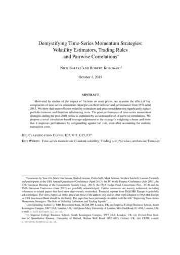
Table 1: Gross Momentum Returns, Unadjusted for Costs (% per Month)Portfolio SizeJan 1992-Dec 2010SP5000.6311.15MaxMinMedianMonthly St Dev.CorrelationOutperform 06; 4.303.462.64-3.224.243.302.84-3.014.20Portfolio SizeJan 1992-Dec 2010MaxMinMedianMonthly St Dev.CorrelationOutperform 06; 09-102345672.68*** 2.94*** 2.95*** 3.04*** 3.04*** 3.07***891015203040503.06*** 2.91*** 2.82*** 2.54*** 2.36*** 2.28*** 2.20*** 2.063.002.541.88-2.122.922.531.74-2.122.83Note: For the analysis, a six-month formation period (-5 to 0 months) is implemented, ranking each stock by itsformation period (six-month) performance, from best to worst. After ranking each stock, equally weightedportfolios were formed that contained the best (1, 2, 3, 4, 5, 6, 7, 8, 9, 10, 15, 20, 30, 40, 50) performing stocksin the formation period. We established a 12-month holding period and the overall return of each time periodwas calculated by averaging the performance of all stocks in each portfolio. Over multiple time periods, theaverage annual total return (geometric mean) of each portfolio was calculated in order to reach the monthly grossreturns. Correlation is between each portfolio and the S&P 500. "Outperform S&P 500" means the percentage ofmonths where each portfolio outperforms the S&P 500 benchmark. Statistical significance of the overall returnsis given by two sample parametric t-tests comparing the returns of each portfolio with the S&P 500.* Significant at the 10% level, ** significant at the 5% level, *** significant at the 1% level.The results in Table 1 show that all portfolios, on average, outperform the S&P 500benchmark by 0.52%-2.44% per month. 12 Consistent with Siganos (2007), larger momentumprofits were primarily seen in the smaller portfolios. However, the portfolio containing the12The S&P 500 was used as the benchmark in this analysis as it the most commonly used benchmark for U.S.stocks. We also ran the risk analysis against the Willshire 5000 Index, arguably a more comparable benchmark,and found similar results.8
best performing stock performed the worst out of all portfolios (1.15%), which is inconsistentwith the findings of Ammann, Moellenback, and Schmid (2011) and with those of Rey andSchmid (2007). Overall portfolio performance gradually increases until it reaches the highestperformance, 3.07% per month, in the top seven stock portfolio. The returns then decrease asthe portfolio holds more stocks. Regardless, the top 50 stock portfolio still outperformed theS&P 500 by 1.50% per month in the overall sample period.Gross returns were divided into two equal sub-periods, January 1992 to December 2000 andJanuary 2001 to December 2009. Each sub-period appears to consistently outperform the S&P500 in both categories. However, momentum trading clearly struggled during the financialcrisis of 2007 and 2008, incurring heavy losses and faring much worse than the S&P 500. Inthis period, all portfolios underperformed the S&P 500 by 0.54% in the top 50 portfolio, andby as much as 2.74% per month in the one stock portfolio. These findings are consistent withAndrikopoulos, Clunie, and Siganos (2013), who find no evidence of momentum returnsduring a similar period, February 2007 to February 2010, in the U.K. market. In hindsight, itwould have been more profitable to either stay in cash or seek an alternative tradingstrategy. 13 We hope that these findings inspire further research into whether it is possible tocapture reliable ex-ante cues from the formation period data that can inform investors as towhether they should continue with the momentum strategy or opt for an alternative tradingstrategy for those holding periods.3.2 Transaction CostsTo more accurately analyze the true profitability of momentum trading, all applicabletransaction costs are applied to each portfolio. At the beginning and end of each holdingperiod, a flat 10 commission per trade was factored in for each buy and sell order.13Daniel and Moskowitz (2013) find that in extreme market environments, the loser portfolio provides a highpremium, while the winner portfolio returns are minimal following large market declines.9
The bid and ask spreads were also taken into account for each stock. The actual bid and askspreads for the stocks were available only from April 2006 to December 2010. Therefore, weimplemented averaged bid and ask spreads based on the market capitalization of each stock,using the bid/ask spread averages from small, mid, and large cap stocks listed on the NYSE in1998 (Bessimbinder, 2003). Specifically, for all stocks with a market capitalization under 215.6 million we assume a 0.750% half spread on both the buy and sell order each period. Ahalf spread of 0.497% was used for stocks with market capitalization between 215.7 and 11,365.8 million. All stocks with a market capitalization greater than 11,365.8 million weregiven a half spread of 0.212%. 14 For the top 50 performers over the 18-year sample period,31% of the stocks were classified as small capitalization, 65% were mid-capitalization, and4% were large capitalization. Although the lack of actual bid and ask data was not ideal, thecurrent market is so heavily traded that every stock ranked in the top 10 best performingstocks for all 12 formation periods in 2010 had an average bid and ask spread of .01,providing a more favorable trading environment for investors seeking to implement thisstrategy in the future.Finally, a nominal “Securities and Exchange Commission (SEC) Fee” for every sale of astock was included at its rate, prior to December 28, 2001, 0.003333% of the total amountsold. 1514These assumptions are supported by the available bid/ask spread data from April 2006 to December 2010.During this time span, the average actual small cap stock posted a half bid/ask spread of 0.65%, which is slightlyless than our assumed average. The mid cap and large cap stocks posted significantly lower actual bid/ask halfspreads, 0.19% and 0.10%, respectively. As a robustness check, we ran the analysis with the actual spreads ofthe relevant stocks for this period and found no systematic difference from the results in our base scenario withfixed spreads for small, mid, and large caps.15Section 31 of the Securities Exchange Act of 1934 states that, “self-regulatory organizations (SROs) such asthe Financial Industry Regulatory Authority (FINRA) and all of the national securities exchanges (including theNew York Stock Exchange) must pay transaction fees to the SEC based on the volume of securities sold on theirmarkets. These fees recover the costs incurred by the government, including the SEC, for supervising andregulating the securities markets and securities professionals.” Viewed on 05.03.2014 on athttp://www.sec.gov/answers/sec31.htm.10
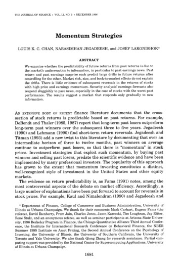
To maintain an equally weighted portfolio at the beginning of each holding period, allportfolios were rebalanced at the end of the previous holding period. Therefore, at the end ofthe holding period, the full 10 commission for each stock, the other half bid/ask spread, andthe SEC selling fee were added to the full amount of the sell order of each stock. In summary,the overall costs, o, to implement a 12-month momentum strategy are:𝑜𝑜 (2 𝑐𝑐) (2 0.5𝑠𝑠) 𝑓𝑓(1)Where c is the sales commission, s is the bid/ask spread, and f is the SEC sales fee.These transaction costs are applied to nine different initial investment amounts ranging from 5,000 up to 1,000,000 in order to reflect the feasibility and effects on performance.Table 2 shows the net monthly returns after applying transaction costs. With a tradingfrequency of only once per year, all (except one) portfolios continued to outperform the S&P500. 16 Yearly traded portfolios containing the top five to eight stocks continue to generate thehighest gross returns, ranging from 2.66% to 2.96% per month. No expenses were added tothe S&P 500 benchmark in this section, which further strengthens the results.16The top 50 stock portfolio with an initial amount of 5,000 underperformed the S&P 500 by 0.39% per month.11
Table 2: Net Monthly Momentum Returns After Adding Transaction Costs (%) Full Turnover; Yearly Trading FrequencyS&P 500 Return: 0.63Initial /# Stocks123456789101520304050 5,0001.07 2.52*** 2.71*** 2.67*** 2.74*** 2.70*** 2.69*** 2.66*** 2.47*** 2.34*** 1.89*** 1.54*** 1.11*0.670.24 10,0001.09 2.57*** 2.77*** 2.76*** 2.84*** 2.82*** 2.83*** 2.81*** 2.65*** 2.53*** 2.16*** 1.91*** 1.65*** 1.40*** 1.15** 15,0001.10 2.58*** 2.79*** 2.78*** 2.87*** 2.86*** 2.87*** 2.86*** 2.70*** 2.60*** 2.26*** 2.03*** 1.83*** 1.64*** 1.44*** 30,0001.11 2.60*** 2.81*** 2.81*** 2.91*** 2.90*** 2.92*** 2.91*** 2.76*** 2.66*** 2.35*** 2.15*** 2.01*** 1.87*** 1.74*** 50,0001.11 2.60*** 2.82*** 2.82*** 2.92*** 2.91*** 2.94*** 2.93*** 2.78*** 2.68*** 2.38*** 2.20*** 2.08*** 1.97*** 1.86*** 100,0001.11 2.61*** 2.83*** 2.83*** 2.93*** 2.92*** 2.95*** 2.95*** 2.80*** 2.70*** 2.41*** 2.23*** 2.13*** 2.04*** 1.95*** 250,0001.12 2.61*** 2.83*** 2.83*** 2.94*** 2.93*** 2.96*** 2.96*** 2.81*** 2.71*** 2.43*** 2.25*** 2.16*** 2.08*** 2.00*** 500,0001.12 2.61*** 2.83*** 2.84*** 2.94*** 2.93*** 2.96*** 2.96*** 2.81*** 2.72*** 2.43*** 2.26*** 2.17*** 2.09*** 2.02*** 1,000,0001.12 2.61*** 2.83*** 2.84*** 2.94*** 2.93*** 2.96*** 2.96*** 2.81*** 2.72*** 2.44*** 2.26*** 2.18*** 2.10*** 2.02***Note: Full turnover applies the commission ( 10 per stock) and half bid/ask spread at the beginning of each holding period. At the end of the holding period, the fullturnover applies the full commission for each stock, the other half bid/ask spread and the SEC selling fee on the full amount of the sell order of each stock. Statisticalsignificance is given by two sample parametric t-tests comparing the returns of each portfolio with the S&P 500.* Significant at the 10% level, ** significant at the 5% level, *** significant at the 1% level.12
3.3 Real TurnoverIt is possible that, when turning over the portfolio from one holding period to the next, anindividual stock could remain in the portfolio. In this case, the overall portfolio would stillneed to be rebalanced, requiring a buy or sell order for a fraction of this stock position, inorder to maintain an equally weighted portfolio at the beginning of each holding period. Thus,one 10 commission would still be applied for each stock. However, the second commissionof 10 is saved in this instance as only one transaction is needed for the adjustment.Moreover, as only a fraction of the stock position would be bought or sold for rebalancingpurposes, the negative consequences of the bid/ask spread are mostly waived, thereby furtherreducing the overall transaction fees. We make these adjustments so as to reflect the realworld situation as accurately as possible, even though comparing Table 3 (real turnover) withTable 2 (full turnover) shows that the performance effect is negligible. Nevertheless, weconsider the real turnover in all analyses that follow.13
Table 3: Net Monthly Momentum Returns After Adding Transaction Costs (%) Real Turnover; Yearly Trading FrequencyS&P 500 Return: 0.63Initial /# Stocks123456789101520304050 5,0001.07 2.52*** 2.71*** 2.68*** 2.74*** 2.70*** 2.69*** 2.66*** 2.48*** 2.35*** 1.89*** 1.55*** 1.11*0.680.25 10,0001.10 2.57*** 2.77*** 2.76*** 2.84*** 2.82*** 2.83*** 2.81*** 2.65*** 2.53*** 2.17*** 1.91*** 1.65*** 1.40*** 1.15** 15,0001.10 2.58*** 2.80*** 2.79*** 2.88*** 2.86*** 2.88*** 2.86*** 2.71*** 2.60*** 2.26*** 2.03*** 1.83*** 1.64*** 1.45*** 30,0001.11 2.60*** 2.82*** 2.81*** 2.91*** 2.90*** 2.92*** 2.91*** 2.76*** 2.66*** 2.35*** 2.15*** 2.01*** 1.88*** 1.74*** 50,0001.11 2.60*** 2.82*** 2.82*** 2.92*** 2.92*** 2.94*** 2.94*** 2.78*** 2.69*** 2.39*** 2.20*** 2.08*** 1.97*** 1.86*** 100,0001.12 2.61*** 2.83*** 2.83*** 2.93*** 2.93*** 2.95*** 2.95*** 2.80*** 2.70*** 2.41*** 2.23*** 2.14*** 2.04*** 1.95*** 250,0001.12 2.61*** 2.84*** 2.84*** 2.94*** 2.93*** 2.96*** 2.96*** 2.81*** 2.72*** 2.43*** 2.26*** 2.17*** 2.08*** 2.00*** 500,0001.12 2.61*** 2.84*** 2.84*** 2.94*** 2.94*** 2.96*** 2.96*** 2.82*** 2.72*** 2.44*** 2.26*** 2.18*** 2.10*** 2.02*** 1,000,0001.12 2.61*** 2.84*** 2.84*** 2.94*** 2.94*** 2.97*** 2.96*** 2.82*** 2.72*** 2.44*** 2.27*** 2.18*** 2.11*** 2.03***Note: Net monthly momentum returns, reflecting the real portfolio returns for those stocks remaining in each portfolio from one holding period to the next. Thus, acommission of 10 is saved in this instance as a new stock is not required to be purchased for the next holding period. Moreover, as only a fraction of the stock holdingwould be sold for rebalancing purposes, the negative consequences of the bid/ask spread would be waived, thereby further reducing the overall transaction fees.Statistical significance is given by two sample parametric t-tests comparing the returns of each portfolio with the S&P 500.* Significant at the 10% level, ** significant at the 5% level, *** significant at the 1% level.14
3.4 Risk FactorsThis section applies the net monthly results from the previous section to various risk factors inorder to determine if these returns continue to outperform the benchmark after factoring inrisk. The capital asset pricing model (Sharpe, 1964) and the Fama-French three factor model(1993) are applied to the net monthly returns of each portfolio in order to test againstsystematic risk.For the capital asset pricing model (CAPM), overlapping data were used in the sample set. Amajority of recent finance literature employs overlapping data (Harri & Brorsen, 2009),although there is no consensus on which type of data are less biased. To control for theautocorrelation of the overlapping data, the Newey-West (1987) estimator with an 11-monthlag was applied. For our estimation, we use the following equation:𝑁𝑁𝑁𝑁 𝑅𝑅𝑓𝑓 β ( 𝐾𝐾𝑚𝑚 𝑅𝑅𝑓𝑓
Jegadeesh and Titman (1993), assumes a zero-cost trading strategy, omits various which market frictions, such as sts, bidtransaction coask spreads, and short- -selling constraints. Carhart (1997) concludes that momentum trading, as proposed by Jegadeesh and Titman (1993), becomes unprofitable after factoring in such trading costs.File Size: 762KBPage Count: 32Explore furtherOption Volatility And Pricing. Sheldon Natenberg.pdf .idoc.pubApplying Deep Learning to Enhance Momentum Trading .cs229.stanford.eduA Unified Theory of Underreaction, Momentum Trading, an www.columbia.eduIlliquidity and Stock Returns: Cross-Section and Time .papers.ssrn.comMarkowitz Theory of Portfolio Management Financial Eco www.economicsdiscussion.netRecommended to you b