WIXLIB

There are no restrictions short selling. There are no transaction costs. All securities are perfectly divisible. There are no dividends during the life of the derivative. The risk-free rate of interest is constant and the same for all maturities.Being c a Call options, and p a put option, their prices according to the Black-Scholes modelare [3]:c S0 e rT (N (d1 ) KN (d2 ))(1)p Ke rT (N ( d2 ) S0 N ( d1 ))(2)whered1 ln 2r σ2 T σ TS0 Kd2 d1 σ Tand N (x) is the standard normal cumulative distribution function given byN (x) 12πRx ex22dx.The price of an option depends on the price of the underlying, the strike price, the risk freerate, and the implied volatility.2.5Decomposition of a portfolio profits and losses (P&L) in its greeks componentsSuppose that at t0 we build a portfolio V0 made of one option, whose price P (S, t, σ, r) is obtainedusing the back scholes model.When time passes from t0 to t1 (4t t1 t0 ) the portfolio s P&L is 4V V1 V0 , theunderlying would have moved 4S S1 S0 , and the implied volatility 4σ σ1imp σ0imp . Wecan decompose the P&L using a first order Taylor expansion:14P δS ν4σ imp θ4t Γ(4S)22(3)Where Delta (δ) is the first derivative of the price with respect to the underlying, Vega (ν) isthe first derivative of the price with respect to the implied volatility, Theta (θ) the first derivative of the price with respect to the time to expiration, and Gamma (Γ) the second derivative ofthe price with respect to the underlying. It can be easily shown that for a geometrical brownianmotion (4S)2 4t [3], therefore all the terms are first order.δ,ν,Γ and θ are the so called ”Greek letters”, and they represent the sensitivity of the option priceto a single-unit change in the value of either a state variable or a parameter. Such sensitivitiescan represent the different dimensions to the risk in an option. The greeks of the combinationof options are the sum of the individual greeks, and each combination has its own risk profile.Delta can be interpreted as the probability that an option will end up in the money.7

The Theta of an option is defined as the rate of change of the value of the option with respectto the passage of time with all else remaining the same. Theta is sometimes referred to as thetime decay of the option, the change in the price of the option for a 1-day decrease in the timeremaining to expiration.The Vega of an option is defined as the rate of change of the value of the option with respect tothe implied volatility of the price.From equation 1, for a call option, the greeks can be obtained straightforwardly [3].: e rT N (d1 ),S0 N 0 (d1 ) rKe rT N (d2 )σ T ν S0 T N 0 (d1 )e rf TΘ Γ N 0 (d1 ) .S0 σ TThe greeks of a put option can be obtained in the same fashion.A portfolio λ made of an option minus delta times the underlyng:λ {O δS}(4)is said to be delta hedged, since the delta component of the option price is offset by theunderlying. This is true as long as the linear approximation implied in equation 3 holds. Usuallydelta hedged portfolios have to be adjusted one or two time a day, to remain hedged.8

3Vertical spreadsA vertical spread can be defined as the linear combination of long calls and short calls or shortputs and long puts, having the long options the same strike price K (long leg) and the shortoptions a different strike price K (short leg). The expiration time is the same for all the optionsthat conform the spread. If a vertical spread is conformed by the same number of long andshort options, it is called a ”pure” vertical spread, otherwise it is a ratio vertical spread. Inthis document we will study pure vertical spreads, and we will refer to them simply as verticalspreads.As defined before, a vertical spread has always a long leg and a short leg. At expiration, avertical spread will have a minimum value of zero, when both options are out of the money(OTM) and a maximum value of the amount between strike prices, when both options are inthe money (ITM).According to the strike of each leg, we can classify the vertical spreads into4 types: bullish call spread, bullish put spread, bearish call spread and bearish put spread [1].The payoff of every diferent type of spread is obtained by adding the the payoff of its constituentoptions, and are represented in (Figure6) and (Figure7)Figure 6: Value of a bullish call or bullish put at expirationFigure 7: Value of a bearish call or bearish put at expirationBeing K and K the strikes (K K ), and Pl and Ps the absolute value of the prices ofthe long and the short leg respectively, the classification can be summarized in Table 1.9

Table 1: Different kind of spreads that can be built with the strike prices K and K beingK K , together with their maximum profits and losses.Long leg strikeShort leg strikeMaximum profMaximum lossBullish call spreadBullish put spreadK K K K (Pl Ps )Pl PsK K Ps PlK K (Ps Pl )BearishcallspreadK K Ps PlK K (Ps Pl )BearishputspreadK K K K (Pl Ps )Pl PsOther authors [2] classify vertical spreads according to wether you get money o give moneywhen you enter in the spread. For example, for a call option, price decreases with strike [3]therefore, entering a bullish call spread costs Pl Ps whereas entering a bearish call spread givesPs Pl . In general, regular traders use vertical spreads when they have a directional view onthe market and they dont want volatility to be there primary concern [1].4Greeks analysis of vertical spreadsIn this section, we show the analytical expressions of the greeks for each type of vertical spread,and we analyze their implications. We assume two general strike prices, K1 and K2, whereK2 K1, a spot price S, an implied volatility σ, and time to expiration t.We also show graphically (Figures 8,9,10 and 11) the evolution of the price and the greeks asa function of time and spot price, corresponding to all the different vertical spreads that canbe built using the strikes K1 1000 and K2 1100. All the calculations were done assumingσ 30%, a risk free interest rate r 2.8% and time to expiration 30 days t 30/360 0.0833in agreement with previously recorded market data.10

4.14.1.1Bullish call spread.DeltaDelta, for this type spread, is expressed mathematically as:δ e rt [N (d1) N (d2)](5) Where t is time to expiration, d1 [ln(S/K1) 12 σ 2 t]/σ t, d2 [ln(S/K2) 12 σ 2 t]/σ t andN (x) is the cumulative probability distribution function for a standardized normal distribution.Since K2 K1 then d1 d2 and N (d1) N (d2), therefore delta is always positive, and thespread always has a bullish perspective.For n(d2)/n(d1) K2/K1, delta is maximized (this expression can be derived by making thepartial derivatives of δ with respect to K1 and K2, and matching both expressions, since at themaximum they are equal to 0).4.1.2GammaGamma, for this type of spread, is expressed mathematically as:Γ 1 (n(d1) n(d2))Sσ t(6)Where n(x) is the standardized normal probability density function. Gamma is zero whenn(d1) n(d2). Since the standardized normal density function is symmetrical around 0, the 1 2former expression is fulfilled when d(1) d(2), which implies that K1K2 Se 2 σ t .When entering the spread, the trader can choose wether to be long or short in gamma adjustingthe strike prices of the legs. The highest gamma values are achieved when n(d1) is in itsmaximum, setting n(d2) as lower as posible. n(d1) is in its maximum when d1 0 which1 2implies that K1 Se 2 σ t . Setting K2 as out of the money as possible minimizes n(d2).Close tothe expiring date, gamma ”explodes” since t is dividing.4.1.3VegaThe analytical expression for vega is ν Se rt t(n(d1) n(d2))(7) 1 2Like in the gamma case, vega is zero when n(d1) n(d2) and K1K2 Se 2 σ t . Vega is also1 2maximum for K1 Se 2 σ t and setting K2 as higher as possible minimizes n(d2). The furtherthe expiration date, the higher is vega.4.1.4”Singular” point 1 2At K1K2 Se 2 σ t gamma, vega and theta are zero. Entering the spread in that position is,for a sufficiently short period of time, equivalent to enter a pure delta position. In the case of1 2K1 1000, K2 1100, r 2.8%, t 30/360 and σ 30% we obtain e 2 σ t 1.0003, thereforeS K1 K2 1048 K1 K2 K1211

4.1.5GraphsFigure 8: Evolution with time and spot of the price and the greeks of a bullish call spread with shortleg strike K2 1100, long leg strike K1 1000, vol 30% and r 2.812

4.2Bullish put spread.The greeks of the bullish put spread are equal to the greeks of the bullish call spread.Figure 9: Evolution with time and spot of the price and the greeks of a bullish put spread with shortleg strike K2 1100, long leg strike K1 1000, vol 30% and r 2.8.13

4.34.3.1Bearish call spread.DeltaDelta, for this spread, is expressed mathematically as:δ e rt [N (d2) N (d1)](8)Since K1 K2 then d1 d2 and N (d1) N (d2), therefore delta is always negative, andthe spread always has a bearish perspective.For n(d2)/n(d1) K2/K1, delta is minimized (this expression can be derived by making thepartial derivatives of δ with respect to K1 and K2, and matching both expressions, since at themaximum they are equal to 0)).4.3.2GammaGamma, for this spread, is expressed mathematically as:Γ 1 (n(d2) n(d1))Sσ t(9)Gamma is zero when n(d1) n(d2). Since the normal density function is symmetrical around 1 20, the last expression is fulfilled when d(1) d(2) which implies that K1K2 Se 2 σ t .When entering the spread, the trader can choose wether to be long or short in gamma adjustingthe strike prices of the legs. The highest gamma values are achieved when n(d2) is in itsmaximum, setting n(d1) as lower as posible. n(d2) is in its maximum when d2 0 which1 2implies that K2 Se 2 σ t . Setting K1 as much ITM as possible minimizes n(d1). Close to theexpirying date, gamma ”explodes” since t is dividing.4.3.3VegaThe analytical expression for Vega is ν Se rt t(n(d2) n(d1))(10) 1 2. Like in the gamma case, Vega is zero when n(d1) n(d2) and K1K2 Se 2 σ t . Vega is1 2also maximum for K2 Se 2 σ t and setting K1 as lower as possible minimizes n(d1). Also thefurther from the exprying date, the higher is gamma.4.3.4”Singular” point 1 2At K1K2 Se 2 σ t gamma, vega and theta are zero. Entering the spread in that position is,for a sufficiently short period of time, equivalent to enter a pure delta position.14

4.3.5GraphsFigure 10: Evolution with time and spot of the price and the greeks of a bearish call spread with shortleg strike K1 1000, long leg strike K2 1100, vol 30% and r 2.8.15

4.4Bearish put spread.The greeks of a bearish put spread are equivalent to the greeks of bearish call spread.Figure 11: Evolution with time and spot of the price and the greeks of a bearish put spread with shortleg strike K1 1000, long leg strike K2 1100, vol 30% and r 2.8.4.54.5.1Influence of volatility on the spreadsLow implied volatility scenarioLets assume that at t0 we want to enter into a bearish call vertical spread and that the impliedvolatility of the options is low. We expect that at t1 the implied volatility suffers an upwardsshift of 300 basis points. We have taken the data of two bearish spreads from the data baseBloomberg, and we have calculated how the shift of the implied volatility affect their prices (table2). Since the aim of the section is to compare the sensibility to changes in implied volatility of2 similar spreads, we set aside the effects of delta, theta and gamma, by keeping constant t, andS. The days to expiration at t0 are 18, t1 t0 1 day, the interest rate is 0.219%, and the spotprice is S 1187.00 (S&P 500 mini futures).16

Table 2: Evolution of the price of to bearish calls (the price is given in units of the underlying(u), to calculate the price in dollars, the number must be multiplied by the nominal value of thecontract), when there is a downwards shift of 3 % of the implied volatility level. For the bearishcall 1 the short leg is initially ATM and the long leg is OTM, whereas for the bearish call 2 theshort leg is initially ITM and the long leg is ATMBearish call 1Bearish call 2Short leg strike (K1)and implied vol at t0K1 ATMσi 29.496%K1 5%ITMσi 33.565%Long leg strike (K2)and implied vol at t0K2 4.21% OTMσi 26.727%K2 ATMσi 30.710%Price at t0P&L-20.75uPrice at t14σ 3%-21.31u-32.83u-32.33u0.5u-0.56uAs we have seen in section 2.3.3, for a bearish call spread, the maximum sensitivity to vega1 21 2is achieved when the higher strike (long leg) is at K2 Se 2 σ t . In this case: e 2 σ t 1.0002 1hence, the closest is the long leg to the ATM position, the longer in implied volatility is thespread. For these reason, the spread 2 earns money under an hypothetical 3% increment involatility while the spread 1 does not.4.5.2High implied volatility scenarioUsing the same parameters as in section 3.6, lets assume that at t1 the volatility will suffer adownwards shifts of 300 basis points (table 3).Table 3: Evolution of the price of to bearish calls, when there is a downwards shift of 3 % of theimplied volatility level(the price is given in units of the underlying (u), to calculate the price indollars, the number must be multiplied by the nominal value of the contract). For the bearishcall 1 the short leg is initially ATM and the long leg is OTM, whereas for the bearish call 2 theshort leg is initially ITM and the long leg is ATMBearish call 1Bearish call 2Short leg strike (K1)and implied vol at t0K1 ATMσi 29.496%K1 5%ITMσi 33.565%Long leg strike (K2)and implied vol at t0K2 4.21% OTMσi 26.727%K2 ATMσi 30.710%Price at t0P&L-20.75uPrice at t14σ 3%-20.05u-32.83u-33.10u-0.27uAs we have seen in section 2.3.3, for a bearish call spread, the maximum sensitivity to vega1 21 2is achieved when the higher strike (long leg) is at K2 Se 2 σ t . In this case: e 2 σ t 1.0002 1,the closest is the long leg to the ATM position, the longer in implied volatility is the spread.For these reason, the spread 1 earns money under an hypothetical 3% decreasing in volatilitywhile the spread 2 does not.170.7u

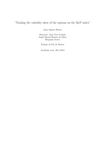
5The volatility smileOne of the main assumptions of the Black Scholes options pricing model is that the mechanicsof the underlying of an option are ruled by a geometrical brownian motion, hence with volatilityindependent of strike prices, spot prices, or time to expiry (variance goes with t in this kindof motion).The implied volatility in the prices of options prior to October 1987 was in agreement with theformer assumption. Until then a plot of the implied vol vs the strike price, or the spot price,showed a straight horizontal line, or a straight horizontal plane in the case of plotting the impliedvol vs the strike prices and the time to expiry.In october 1987 the stock market drop by 20 % or more in two days. This kind of extrememovements conform what is usually called the ”heavy tails”, and are not taken into account ina geometrical brownian motion model. After this, the markets reacted making more expensivelow strike puts than high strike or ATM calls. By doing this, a speculator pays more for a deepOTM strike put, since a extreme favorable movement, with neglige probability in the BSM, isindeed possible. Since then the plot of the implied volatility vs strike prices, resembles a skewor even a smile, depending also on the time to expiration (Figure 12).Figure 12: The implied volatility values of the calls on the S&P Index expiring on December 2011 areplot vs the moneynes.We define the moneyness of an option as m K/S expressed in points per cent,where K is the strike price of the option and S the underlying Spot price. The expiration time is 6 monthsand two weeks. It is said that the shape is a skewEach market has developed its own ”idiosincratic” volatility smile. Until ”the advent” of andalternative model to the BSM, options are priced using BlackScholes, but the implied volatilityof the price is adjusted to the volatility smile of the particular option market.In this section we show the specific properties of the volatility skew associated to the optionsthat we use to make the strategy. To do this we used a set of historical data taken from thedatabase Bloomberg, with the following characteristics: Calls on the S&P 500 mini futures thatexpire in December 2011. The first sample corresponds to the 1st of june, and the samplingfrecuency is 20 min18

5.1Features of the volatility smile of equity index optionsIn this section we enumerate the general features of the volatility smile according to [7], and wetest them using our historical data.5.1.1”Volatility are steepest for small expirations as a function of strike, shallowerfor longer expirations”This feature can be clearly seen in the historical data.Let us define the moneyness of an option as m K/S expressed in points per cent, where K isthe strike price of the option and S the underlying Spot price. In figure 13 we show the evolutionof the slope (β) of the skew, directly measured from the m 95% and the m 90% optionsusing the following expression:β(ti ) σ95 (ti ) σ90 (ti )(95 90)(11)Figure 13: Evolution of the slope (β), calculated according to the equation (7) as function of time toexpiry. In the same graph the moving average, the moving average moving standard deviation and themoving average - moving standard deviation can be found. This statistics were calculated according toequation 12 and equation 13The moving average was calculated using the following expressionsPn iM A(ti ) n (i 31) β(tn )30The standard deviation was calculated using the following expression19(12)

vuu1M S(ti ) t30n iX(β(tn ) M A(ti ))2(13)n (i 31)The graph of figure 13 also shows another feature: The volatility of the volatility ishigher the closer is the option to expiration5.1.2”There is a negative correlation between changes in implied ATM volatilityand changes in the underlying itself”In figure 14 we show the ”ATM volatility vs time” graph together with the ”underlying vs timegraph” for our historical data.The negative correlation can be clearly seen.Figure 14: Up:Implied volatility of the ATM options, as a function of the time to expiry. Down: Spotprice of the underlying, as a function of the time to expiryThe value of the Pearson correlation coefficient isρ 0.9170(14)Since index is formed by the sum of n stocks Xi , the variance of the index is given by theexpression:var(nXi 1Xi ) nXvar(Xi ) 2i 1n XnXi 1 j i 120cov(Xi , Xj)(15)

When the market drops, the correlation between the stocks increases, increasing also thevolatility of

an in-the-money option is S Kfor calls, and K Sfor puts, and the intrinsic value of out of the money options is always 0. The di erence between the option value and the intrinsic value is the time value of the option, time value represents the additional value of an option due to the opportunity for the intrinsic value of the option to increase.