WIXLIB

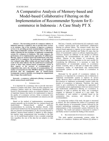
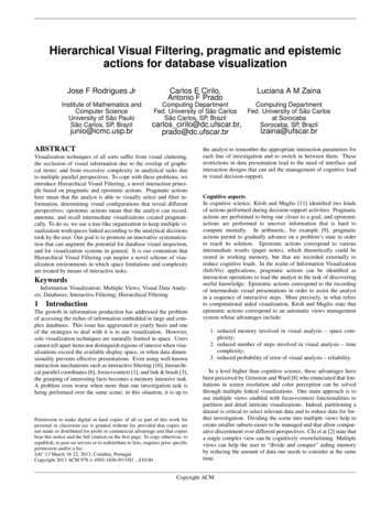
28th Annual ACM Symposium on Applied Computing, 20132Visualizing relational databasesIn the last decade, many works have addressed the issue of visualizing relational databases to formulate new hypotheses, to validate known hypotheses, or to simply present facts more intuitively.These works include multivariate multiple-view systems, and relational database driven systems.Among the multivariate multiple-view systems, the GGobi system [4], and the Xmdv tool [17] employ linked views as definedby the Link & Brush principle. Our work differs from these former proposals by means of the hierarchical visual filtering principle. For this reason, our work cannot be directly compared to theseother proposals, due to its innovative interaction scheme, and to itsdatabase orientation.More specific to our work, in the field of relational-databasedriven systems, Wang et al. [20] present the ZoomTree, a webbased system that uses a grid layout to present sequential zoomoperations carried over a database. Different from our approach,the ZoomTree allows data propagation via selection of dimensionsto draw aggregation datacubes; also, the selection of data does notfollow free database querying, instead, it is restricted to datacuberefinement operations. A pioneer work on the same topic is systemPolaris [18], another grid-based layout whose main feature is itsflexibility in defining the visual encoding; different from our work,Polaris does not allow hierarchical exploration, rather it improveson the commercial Pivot Table method. Another related proposalis the work of Mansmann and Scholl [12]; their DecompositionTree permits the user to visually conduct datacube operations, thatis, dimension-oriented operations that are data-driven, rather thananalysis-driven. As a last remark, we can state that our work isdefined over a combination of visualization with clutter reductiontechniques; in this scenario, even if we consider the taxonomic review of clutter-reduction techniques of Ellis and Dix [5], we findthat our interaction scheme is a novel contribution.Visual filteringVisual filtering (or brushing) over multiple coordinated views [15]is one of the main interaction techniques for visualization; it allows analysts to select the graphical items that are more interesting, gaining focus and details over them. In a recent work,Weaver [22] introduces a scheme that is opposite to ours. Insteadof creating multiple views by means of visual filtering, they definea collective filtering based on selections originating from multipleviews. Kehrer et al. [10] argue in favor of statistical summarizations (mean, variance, skewness, and kurtosis), each in a dedicatedview, as a means for interpreting visually filtered data. Also recent, Turkay et al. [19] create multiple views by simultaneously filtering data and data dimensions assisted by statistical summaries.In another work, Weaver [21] proposes the use of boolean logicto progressively refine the content visually presented, leading to amore robust filtering. Our work differs from all these proposals asit permits an unrestricted number of views that are kept linked bycomplimentary actions; besides, our proposal is adequate for anykind of visualization technique, including statistical summaries aswell.The rest of the text is organized as follows. In section 2 wepresent the innovations proposed by our system along with concepts, analyses, and discussion. In section 3 we formally analyzethe potential of our interaction principle regarding visual clutter. Insection 4 we demonstrate our technique in respect to pragmatic andepistemic actions, just before the final remarks of section 5.MethodologyAs a critical setting for database visual analysis, we consider theuse of heterogeneous visualizations in a multiple views environment making use of pragmatic and epistemic actions. In order toprove this concept, we developed Visualization Tree (VisTree) [13],a system that enables multiple representations of a dataset relationallowing comparison and operation with a strong feeling of locusof control. VisTree is designed for any kind of visualization technique; specifically for this work, we use classical techniques Parallel Coordinates, Scatter Plots, Table Lens [14], and Fastmap-basedprojection [7]. Over the VisTree systematization we demonstratethe Hierarchical Visual Filtering principle.2.1Hierarchical Visual FilteringA straightforward way to partition a dataset is to use relationaldatabase queries that, over visualization scenes, correspond to interactive filtering, a well-known pragmatic instrument of visualization. Extending this interactive principle, here we propose what wecall Hierarchical Visual Filtering, an improvement of interactivefiltering that brings epistemic possibilities to visual analysis. Hierarchical Visual Filtering allows for pragmatic actions as the analystis able to select parts of the visualization scene; and allows for epistemic actions as the analyst is able to record, annotate, and recallintermediate visualizations created over his pragmatic actions. Hierarchical Visual Filtering contributes to visual analysis research intwo ways: by reducing visual clutter for more scalable analysis; by reducing cognitive loads – specially over memory, for aricher analytical experience.Hierarchical Visual Filtering combines interactive selection andprogressive refinement to permit analytical management in ahierarchically-arranged environment. As presented in Figure 1, it iscomposed of a dataset D, a visualization V , a visualization functionv, an interactive filtering function f and a function Λ that plays justreverse to function v.Figure 1: (a) Components of Hierarchical Visual Filtering, (b)functions that define it, and (c) its iterative cycle.In Figure 1, function v : Di Vi is parameterized by a pair (s, g)where s is the spatialization scheme that states how data D occupythe screen space (projection, graph-like, sequentially, and so on)and g is the set of graphical marks (dots, lines, curves, icons, andso on) used by visualization Vi . Also in Figure 1, filtering functionf : Vi Vi0 is parameterized by a pair (d, e) where d is the set ofdimensions of the data and e is a set of relational select predicatesthat apply to d in order to determine the selection of the interactivefiltering. Interactive filtering produces an altered configuration Vi0that is made of a subset of the graphical entities of visualizationCopyright ACM947

Vi . Function Λ : Vi0 Di 1 receives a filtered visualization Vi0 andperforms the opposite of function v using its same parameters; itreturns the data items Di 1 that define visualization Vi0 .Figure 1 presents the iteration cycle that defines Hierarchical Visual Filtering. According to it, a dataset Di is used to create a visualization Vi through function v. This visualization is interactivelyfiltered via function f to determine a new visualization configuration Vi0 . Then, the data that is being presented in Vi0 is extracted withfunction Λ. With the extracted data Di 1 , a new visualization Vi 1can be created. This process is to be repeated iteratively accordingto the user’s exploratory goals, which determines how many stepsare necessary.In Figure 2, we illustrate the Hierarchical Visual Filtering theway it is performed in VisTree and according to the technique presented in Figure 1. We use two iteration sequences, in the first onethe entire dataset (“SELECT * FROM DATA SET”) D1 is loadedin a new visualization workspace; the interface of this workspacepermits to choose one of five available visualization techniques –Figure 2(a). By choosing one of them, visualization function v istriggered to generate visualization V1 . Over V1 , the user can determine parameters (highlighted in the figure) for interactive functionf , and a new visualization V10 is determined. Another user command (Pipeline – Figure 2(b)) triggers function Λ, which identifiesthe data D2 being presented in V10 (“SELECT * FROM DATA SETWHERE ((139 DIM 2 334) AND (73 DIM 4 78))”).The data of V10 is now sent (pipelined) to a new workspace to createvisualizations V2 and then V20 in the second iteration cycle – Figure2(c).keeping track of the multiple workspaces and to present them in atree-like structure.Figure 3: VisTree Construction. (a) Sequential exploration ofa branch. (b) Parallel exploration over different branches. (c)Iteration at deeper levels of the tree.The epistemic aspect of VisTree comes as the system automatically records the relational predicates used during analysis and,also, it comes as the user is able to annotate each workspace so thatshe/he can remember what the presented data refers to. VisTreecomplements these features by organizing the workspaces in accordance to how they were created, providing a sense of analyticalflow with reduced cognitive load.2.2Figure 2: Hierarchical Visual Filtering iteration loop. (a)Choice for visualization function v; (b) triggering of functionΛ; (c) second iteration cycle.Hierarchical Visual Filtering permits the user to define new visualization workspaces, each one carrying a subset of the data thathe/she considers worthy for analysis. To do this, the user can observe a given workspace and interactively filter its data by choosinga set of parameters e of relational select predicates. When an interesting visualization configuration comes up, the user can commandits data elements to flow to a new workspace. This process canbe repeated for the new workspace or for the same workspace. Asanother workspace is created, the current branch of exploration becomes deeper, as seen in Figure 3(a). If a new workspace is createdfrom the same workspace, a parallel branch of exploration is created, as seen in Figure 3(b). The same operation can be done atany level of the tree, as demonstrated in Figure 3(c). Along thisiteration/interaction, the VisTree systematization is responsible forTree management and interactionAs the user pragmatically creates new workspaces and the treestructure evolves, it is necessary to manage its structure in orderto maximize space utilization and to maintain the epistemic potential of the tree representation. Each node of the tree occupies anequal area of the 2D space, therefore it is necessary to partitionthis space at the same time that the tree representation adjusts to itsspatial arrangement.We developed a recursive algorithm to combine suitable tree presentation with space partitioning of display space. The algorithmuses a tree scheme named tNode – presented in Figure 4(a), whichcarries pointers to son and sibling nodes. It also carries a pointer toan instance of a visualization object, referenced as vis pointer. Thetree data structure grows as the user triggers interaction events, asillustrated in Figures 4(b) and 4(c). The structure is used during thewhole management of the visualization environment.Figure 4: (a) The node structure for managing the VisTree. (b)A tree example and its correspondent data structure. (c) The vispointers hold the instances of the visualizations (workspaces)being presented.Copyright ACM

28th Annual ACM Symposium on Applied Computing, 2013In VisTree, the tree is presented in left to right orientation, instead of top-down as usual. To organize nodes this way, we breakthe node positioning problem in two parts; first, to determine horizontal positioning and, then, to determine vertical positioning. Fora given node, horizontal positioning is straightly achieved using thenode’s (horizontal) level, which corresponds to how deep the nodeis located in the tree, as can be seen in Figure 5. Meanwhile, vertical positioning is a little trickier because it demands positioningfrom the bottom of the display up to its top considering the number of workspaces and of branches at each level. Therefore, treepresentation must start by the leaves, otherwise we may have edgecrossings and/or nodes overlapping that could compromise the treeaesthetics.In Figure 5 we illustrate how the presentation process occurs.The first thing is that, any new node is positioned at the bottom ofthe screen. In steps 1 through 3 in Figure 5, nodes 5 and 6 illustrate the case for nodes without sons: initial bottom positioning,search for the first node above it (surrounded by circle) and thenrepositioning. In steps 4 through 8, nodes 7 and 8 illustrate the casefor nodes with sons; after the first repositioning, it is necessary toperform a second repositioning according to the child nodes (surrounded by an ellipse). For aesthetic reasons, this second repositioning places the father node in a position where both the sum andthe variance of distances for all child nodes are minimized. Thatis, the father node is positioned in the middle height, which rangesfrom its highest son (or grandson) to its lowest son (or grandson).space, because the nodes would have to satisfy spatial constraintscausing them to be smaller than what is practically visible.Our strategy to handle this matter is to provide automatic andmanual interaction mechanisms to explore the visualization environment. Hence, when the tree does no longer fit the screen spaceand a new node is created, we automatically position this last nodeat the center of the screen. With this mechanism we provide asmuch context as possible for the new node; at the same time, weinduce locus of control, because the last user operation is immediately presented to him/her surrounded by the formerly createdworkspaces.But, as we provide endless visualization space, the drawback isthat the tree can be much bigger than the screen space and actingepistemically becomes a usability problem. To tackle with this, wedesigned an interaction scheme enabled with zooming and translation functionalities. These two features aid in the process but, forlarge trees, they may demand excessive interaction steps in orderfor the user to grasp the desired information. Therefore, we alsodesigned a novel interaction scheme with two features, named Instant Focus and Instant Context: Instant Context, Figure 6 (a), works by presenting the entiretree structure no matter how small its nodes become. To doso, the user has to pass the mouse over a desired node andthe tree will be visualized with emphasis over that node. Itbecomes possible to figure out where in the tree structurethe node is located. As the user moves the cursor out of thedesired node, the application returns to the former spatial arrangement; Instant Focus, Figure 6(c), allows the user to pop up a separate window from the tree structure; this new window bearsthe visualization workspace that the user has chosen for focusing. To do so, similarly, the user must pass the mousecursor over the desired workspace. The focus window canoccupy part of the screen space or can be maximized for theentire screen. To return to the VisTree environment, the userhas to pass the mouse cursor out of the boundaries of the focus window or to close the window in case it has been maximized.Instant Focus and Instant Context permits the user to benefit fromfocus context interaction over the VisTree multiple windows environment.Figure 5: VisTree’s nodes positioning. The first illustrationpresents the desired presentation. Following, steps 1 through8 illustrate the positioning of nodes 5 through 8 in order toachieve the desired configuration. For each positioned node, its“first node above” is highlighted with a circle. Child sons thatare considered for repositioning are highlighted with ellipses.2.3Workspaces management and interactionIn the environment of the VisTree, as new epistemic informationis recorded in the form of new workspaces, the tree grows and itsnodes become smaller in terms of screen space. However, the nodesof the tree have a minimum acceptable size, otherwise, too small visualization scenes could not be observed. For this minimum size,we use 2.5 x 1.5 inches, which nearly corresponds to a two-columnarticle illustration. We assume that the screen resolution will always be sufficient to support such presentation size, no matter thetechnique. This minimum size implicates that, at a certain step, thealgorithm can no longer accommodate the tree inside the displayFigure 6: Instant Context shows where in the tree structure anode of interest is located (a). For large trees, normal presentation may hide context and/or detail (b). Instant Focus presentsthe details of a given scene by increasing its window size (c).3Reduction of visual clutterIn this section we formally demonstrate how the refinementpromoted by Hierarchical Visual Filtering deals with overlap ofgraphical items reducing the problems of visual clutter.Problem formalizationInitially, we formalize the concepts of graphical item, screenspace, and screen-space coordinates. We consider that graphicalCopyright ACM949

items refer to any distinct visual mark used for data visualization,screen-space refers to the available display space that a given visualization can use for presentation, and screen-space coordinates, inturn, refer to each position that can be addressed in a given screenspace.The screen-space is naturally discrete in the number of coordinates, no matter whether the domain of the data being presented isdiscrete or continuous. Consequently, the number of coordinatesin screen-space limits the number of graphical items that can bepresented, what varies depending on the data domain that will bepresented.Although the number of possible graphical items can be muchbigger than the number of screen-coordinates, the number ofpossible graphical items cannot exceed the number of screencoordinates. This problem is even worse for graphical itemsthat are bigger than one pixel. This limitation determines thatvisualization techniques suffer from overlap of graphical itemsand, consequently, by visual cluttering. In this context, overlapof graphical items is understood as the mapping of different dataitems to the same screen coordinate; meanwhile, visual cluttering refers to the confused or disordered arrangement that arisesfrom overlap of graphical items, what negatively affects perception.Overlap of graphical itemsFor this topic, we initially formalize the concept of region of interest. For a given visualization technique, a region of interest is asub-area of the screen-space in which a collection of data items isbeing presented. The biggest region of interest is the whole visualization itself, meanwhile, smaller regions of interest are defined viainteractive filtering.Based on these notions, we can develop a formal metric for theoverlapping of graphical items. The overlap can be measured bythe density of elements that map to one same visual coordinate.Therefore, given a workspace composed by the collection D ofdata items, and by the set G of graphical items, the overlap factoris given by the total number of elements mapped to , that is, D ,divided by the total number of graphical items presented in , thatis, G . Then:overlap f actor D data elements mapped to (1) graphical items presented in G The same holds for regions of interest. That is, given a region ofinterest δ , the overlap f actor is given by the total number ofelements mapped to this region, that is, d for d D, divided bythe total number of graphical items presented in this region, that is,g for g G.As presented in Figure 7, the Hierarchical Visual Filtering determines that, given a region of interest δ withoverlap f actor d / g , it is possible to create a new workspace 0 with overlap f actor0 d / G0 . Considering that a regionof interest is always smaller or equal to the screen-space, andconsidering that the workspaces created via pipelining use thewhole screen-space, then, the following inequality is always valid g G0 . This is because a wider screen-space will be available forthe new pipelined workspace and, thus, more graphical items canbe presented. Consequently, overlap f actor0 overlap f actoris always true. In other words, the pipelining operation will alwayscreate new scenes with equal or reduced overlap f actor.Figure 7: Treatment of graphical items overlap via pipeline refinement. (a) A workspace and a region of interest δ (black ellipse) defined with parameters 17.0 AT T RIBUT E6 18.5. (b) The workspace 0 achieved via pipelining of the regionof interest presented in (a). Also in (b), it is clear the increasein the number of graphical items, specially for AT T RIBUT E6.As consequence, in most dimensions not only the overlap factorwas reduced but also the visual clutter in general.4Experiments over pragmatic and epistemicactionsIn this section we demonstrate the possibilities of the HierarchicalVisual Filtering; to do so, we perform experiments over a datasetof agrometeorological data - the Embrapa dataset. The datasethas 9 attributes: precipitation, maximum temperature, minimumtemperature, normalized difference vegetation index (NDVI), water requirement satisfaction index (WRSI), average temperature,potential evapotranspiration (ETP), real evapotranspiration (ETR)and measured evapotranspiration (ETM) collected partly with remote sensors (satellite) and partly with in locus samples from sugarcane plantation regions in Brazil. The data was collected during 82months from 2001 to 2007, so that each record corresponds to thedata collected in a given month for one region. Since there are 5regions: Araraquara (1), Araras (2), Jaboticabal (3), Jaú (4), andRibeirão Preto (5), there is a total of 410 records. In order to testour hypothesis, we proceeded with the following tasks: characterize the 5 regions in relation to all the attributes ofthe dataset; choose two regions of interest in order to draw further visualclues comparatively.The problem here is that the data is organized according to several regions and, although we want to inspect these regions separately, we do not want to use multiple visualization sessions. Multiple sessions would demand managing several windows, or evenpaper annotations. Also, the data is multivariate and it would be interesting to observe it according to multiple kinds of visualizationtechniques put together in a single environment. Lastly, it is desired to select subsets of the data and to summarize them by meansof statistical calculations drawn over each of the visual workspaces,making the comparative analysis faster. In Figure 8, we show a visualization session for these data and for the proposed tasks; theimage was edited for better presentation.The visualization of all the data items over Parallel Coordinates –Figure 8(a) – presents a hard to interpret cluttering of lines. For this,the first step of the analytical process was to define 5 filterings eachcorresponding to a different region. With the filterings we couldcreate 5 workspaces – Figure 8(b) – presented simultaneously andprone to detailed inspection by means of Instant Focus. Next, wewant to characterize the workspaces’ data with a simple statisticaloperation - to do so, we calculate the average of each dimensionat each workspace and proceed by drawing a polyline of averagevalues emphasized in green on top of the Parallel Coordinates –also presented in Figure 8(b). This first round shows that the 5Copyright ACM

28th Annual ACM Symposium on Applied Computing, 2013Figure 8: Definition of an analytical hierarchy of data over the Embrapa dataset. (a) Visualization of all the data items. (b) Interactivefiltering of 5 subsets of the data, with one workspace to each showing a Parallel Coordinates scene. (c) The 5 workspaces, nowvisualized with Fastmap multidimensional projection. (d) Workspace with the 50% records with highest levels of precipitation ofregion 1. (e) Workspace with the 50% records with lowest levels of precipitation of region 1. Each workspace carries details of itscorrespondent select predicate, number of records, and user annotations (header of each window).regions have similar values for each of the attributes with slightvariations that confer them local peaks according to each averagepolyline.In a next step, we want to visualize the same data in a multidimensional projection achieved using the well-known Fastmap algorithm; as so, in Figure 8(c), another visualization is presented foreach of the workspaces. These new visualizations work by mapping the 9 attributes of the datasets i

database queries that, over visualization scenes, correspond to in-teractive filtering, a well-known pragmatic instrument of visualiza-tion. Extending this interactive principle, here we propose what we call Hierarchical Visual Filtering, an improvement of interactive filtering that brings epistemic possibilities to visual analysis. Hier-