Transcription
Decoherence, the measurement problem, andinterpretations of quantum mechanicsBas HensenDowning CollegeCambridge CB2 1DQ, UKJune 24, 2010
Contents1 The theory of environment-induced decoherence1.1 What is Decoherence? . . . . . . . . . . . . . . . . . . . . . . . .1.2 Basic formalism . . . . . . . . . . . . . . . . . . . . . . . . . . . .1.2.1 Mathematical quantum theory . . . . . . . . . . . . . . .1.2.2 Density operator formalism . . . . . . . . . . . . . . . . .1.2.3 Proper vs. Improper mixtures . . . . . . . . . . . . . . . .1.2.4 Von Neumann ideal measurement scheme . . . . . . . . .1.3 Environment-induced decoherence . . . . . . . . . . . . . . . . .1.3.1 Interaction with the environment . . . . . . . . . . . . . .1.3.2 Environment-induced superselection . . . . . . . . . . . .1.3.3 The quantum measurement limit . . . . . . . . . . . . . .1.3.4 The quantum limit of decoherence and intermediate regime1.3.5 Predictability sieve . . . . . . . . . . . . . . . . . . . . . .1.3.6 Decoherence free subspaces . . . . . . . . . . . . . . . . .1.4 Physical example, realistic models, experimental tests/results . .1.4.1 Free particle localisation due to environmental scattering1.4.2 Double-slit interference . . . . . . . . . . . . . . . . . . .1.4.3 Experimental tests . . . . . . . . . . . . . . . . . . . . . .1.5 Quantum Darwinism . . . . . . . . . . . . . . . . . . . . . . . . .4455710111313141517181819202526272 The2.12.22.32.42.5.303132333434. . . . . . . . . . . . . . . . . . . . . .interpretation. . . . . . . . . . . . . . . . . . . . . . . . . . . . .363740404142444445measurement problemDividing the problem . . . . . . . . . . . .The problems of outcomes and of collapse:The problem of interference: (iii) . . . . .The problem of the preferred basis: (iv) &Quantum to classical transition . . . . . . . . . . .(i) & (ii). . . . . .(v) . . . . . . . . .3 Interpreting quantum theory3.1 Decoherence as an interpretation (?) . . . . . . . .3.2 Other interpretation of quantum theory . . . . . .3.2.1 Standard and Copenhagen interpretation .3.2.2 Wigner/von Neumann quantum mind/body3.2.3 Relative state interpretations . . . . . . . .3.2.4 Modal interpretations . . . . . . . . . . . .3.2.5 de Broglie - Bohm Pilot wave . . . . . . . .3.2.6 Physical collapse theories . . . . . . . . . .4 Summary.471
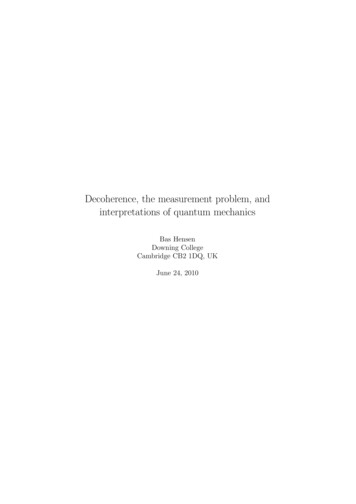
IntroductionConsider a tiny dust-particle of diameter 0,01 mm, floating around in vacuum,and colliding with surrounding photons, illustrated in Figure 1:classical settingquantum settingcoherence bjectPocoherenceΨ objectcoherencecoherencecoherenceFigure 1: The different influence of the environment on the systemin the classical and quantum settings, for a small dust particle immersed in light (photons) from all directions. Left: In the classicalcase, the interaction with the photons does not alter the motion ofthe object. Right: In the quantum case the photons become entangled with the object by the interaction, which causes a delocalisationof the coherence in the object, making quantum effects such as interference patterns unobservable at the level of the system. AfterSchlosshauer[1]In a classical setting, when we consider the movement of the particle, it isperfectly safe to ignore the scattering of the photons. The amount of momentum transferred from the photon to the particle per collision is very small, buteven when the interaction is strong, the incident photons are usually distributedisotropically in position and direction, thus averaging out the momentum transfer to zero. However, in a quantum setting, considering the state of the particleΨ, for instance in the position basis Ψ(x) hx Ψi, generally every collisioninteraction entangles a photon with the particle. In this case the photon distribution does not matter: the initially local coherent state of the particle becomesmore and more entangled with its environment of photons. The photons, flyingoff after scattering, thus delocalise the coherence, which makes quantum effects(such as interference) unobservable at the level of the system. Clearly, in this2
case we cannot just ignore the environment!This is the basic underlying idea of the theory of environment-induced decoherence.It is the purpose of this essay to review the theory of decoherence, and its implications for the traditional problem of quantum measurement, intimately relatedto the emergence of the classical world from a quantum reality. Additionally wediscuss how decoherence fits in with a number of traditional and more recentinterpretations of quantum theory.Roughly, the outline of this essay is as follows: In Chapter 1 I will discuss the physics and mathematics of environmentinduced decoherence, give a few examples of models to which it is applicable, and discuss recent experiments. In Chapter 2 I define the measurement problem (in different ways), discuss why quantum mechanics needs an interpretation, and describe a fewmainstream interpretations of quantum mechanics. Next, combining these two chapters I will discuss the implications of thedecoherence program for the measurement problem itself in Chapter 3;What parts of the measurement problem does the theory (claim) to solve(if any)? Which other interpretations of quantum mechanics connect wellwith results from decoherence theory? Finally I will summarise in chapter 4, including a small outlook from myown perspective.Most of chapter 1 is based on the extensive book on Decoherence publishedby M. Schlosshauer in 2008 [1], and the later chapters use H. Janssen’s 2008master’s thesis [3] as the main source of information.3
Chapter 1The theory ofenvironment-induceddecoherence1.1What is Decoherence?Decoherence is the term used to describe the destruction of phase relations inthe state of a quantum mechanical system, as a result of a dynamical process.According to the Superposition Principle, any two state vectors in a Hilbertspace of a quantum mechanical system, can be linearly added together to formanother valid state of the system: for ψi , φi H Ψi a ψi b φi H(1.1)where a, b C . This causes the occurrence of many purely quantum mechanical effects, such as interference in the double slit experiment (see section 1.4.2),entanglement of quantum systems, and is one of the key reasons a quantumcomputer might be advantageous compared to a classical one [2]. In practicehowever, it is very hard to keep a system in a coherent superposition due tointeractions with its environment, causing interference effects and entanglementcorrelations to vanish quickly. In this basic form, decoherence is then an unwanted but unavoidable fact from perspective of the quantum physicist, in hisattempt to exploit these phase relations in experiments.1However, “decoherence” is now often used for a much more general idea,namely that of the environment-induced decoherence program, referring notonly to the effect of decoherence itself, but also referring to its main cause, the ubiquitous and almost unavoidable interaction of aquantum system with its environment; its physical implications, expressed in predictions for empirically verifiableexperiments;1 Intextbooks related to quantum computation, decoherence is often called quantum noise,or, in the field of quantum information theory, described by a phase damping channel, aprocess in which information is lost without a loss of energy. See for instance [2].4
its conceptual implications, on for instance the traditional problem ofquantum measurement, and the emergence of the classical world from aquantum reality.It is important to distinguish between these last two points, because althoughthe relevance of environment-induced decoherence on empirical outcomes iswidely acknowledged, its conceptual implications are subject to much more controversy. Opinions range from solving (part of) the measurement problem, asfounding decoherence theorists used to claim, to denying any conceptual implications apart from those illustrated any other quantum mechanical calculation.Nevertheless, decoherence theory is a well-established subject, and manycurrently popular philosophical interpretations of quantum theory either useresults from decoherence theory to propagate their ideas, or are entirely basedon these results.1.2Basic formalismThis section contains the basic formalism that we need to describe decoherencein a mathematical formulation of quantum theory. I will describe (very) brieflythe mathematical framework of quantum theory, and the theory of mixed statesand density matrices. We will also look at von Neumann’s Measurement scheme,as it plays a significant role in the philosophical discussion later. Other moreextensive reviews can be found in any quantum theory textbook; this sectionis largely based on the Quantum Information Theory textbook by Nielsen andChuang (2000) [2], and lecture notes by Nilanjana Datta (2009) [4].1.2.1Mathematical quantum theory; Postulates of quantummechanicsQuantum Mechanics is a physical theory that replaces Newtonian mechanicsand Classical Electromagnetism at the atomic and subatomic level. Its mathematical framework can be used to make predictions about the behaviour ofparticular physical systems, and the laws they must obey. The connection between the physical system and a workable mathematical abstraction of it, ismade through a few basic postulates, that were basically derived by a long process of “trail and error”. Note that these postulates are therefore not provenfrom any more fundamental principles. When we come to discuss interpretations of quantum theory and the measurement problem in chapter 2, we have tobe careful not to take these postulates as some kind of absolute truth. Howevermost discussions about interpretation of quantum theory and extensions to itare based on these shared assumptions and we will need them to formulate ourdescription of decoherence.Postulate 1. Any physical system is described by a state vector ψi whichlives in a Hilbert space, a complex vector space equipped with an inner producthφ ψi. A state vector has unit norm hψ ψi 1. In most cases we will encounter, our Hilbert space will simply be Cn ,with ψi being a unit n-dimensional column-vector, with the usual innerproduct.5
This means that any superposition of two state vectors, Ψi a ψi b φi ,(1.2)with a, b C, and a 2 b 2 1, is also a valid state of our system. A property of our physical system that can be measured is called an observable and is represented by a linear operator  acting on H, that isHermitian(self-adjoint):  † .  then has a spectral decompositionP i ai ψi i hψi , where { ψi i} denotes a complete orthonormal set ofeigenvectors of  with corresponding eigenvalues {ai }. We can define theorthogonal projectors P̂i onto the eigenspace of ÂP̂i ψi i hψi ,(1.3)where by definitionP̂i Pˆj δij P̂i ,†P̂i P̂i ,XP̂i Î,(1.4)iwith δij the Kronecker delta, and Î the identity operator. Note that theprojectors themselves have eigenvalues 0 and 1. We will see the significanceof these projectors when we discuss quantum measurement at the thirdpostulate.Postulate 2. The time-evolution of an isolated (closed) quantum system isdescribed by a unitary transformation. ψ(t)i Û (t0 , t) ψ(t0 )i, where Û is aunitary operator acting on H. The unitary transformation Û is determined by solving the Schrödingerequation,d ψi Ĥ ψi ,(1.5)i dtwhere is Planck’s constant, and Ĥ is a linear Hermitian operator actingon H called the Hamiltonian. If Ĥ is time independent, we have iÛ (t0 , t) expĤ(t t0 ) ψi .(1.6) If we are able to construct a general Hamiltonian, we can perform arbitraryunitary transformations on our system. The above relation only holds for isolated systems. However, when anexperiment is done to find out properties of a system, we have to let thesystem interact with our experimental equipment, so the system is nolonger closed and the evolution no longer unitary. The following posulatedescribes the evolution of a system under a measurement.Postulate 3. This postulate is also known as the collapse postulate. Quantummeasurements are described by a collection {M̂m } of linear measurement operators, acting on H, which satisfy the relationX†M̂mM̂m Î.(1.7)mThe index m refers to the measurements outcomes that may occur in the experiment.6
Suppose the system under measurement is in state ψi just before themeasurement. Then the probability of obtaining result m from the measurement is given by†p(m) hψ M̂mM̂m ψi ,(1.8)and the state after measurement is given byM̂m ψi. ψi ψ 0 i q†hψ M̂mM̂m ψi(1.9) Note that the projectors P̂i we defined for observable  of a system in postulate 1 in equation (1.3) satisfy the relation for measurement operators,equation (1.7). All measurements with operators satisfying both (1.7) and(1.4) form an important special case of the general measurement postulate,called projective measurements 2 .Postulate 4. The state space of a composite quantum system made up of two(or more) distinct physical systems is the tensor product of the state spaces ofthe component physical systems. Suppose we have systems numbered 1 throughn, with system number i prepared in the state ψi i, then the composite systemis described by a state vector Ψi which lives in a Hilbert space H H1 H2 . Hn , and is itself given by a tensor product: Ψi ψ1 i ψ2 i . ψn i .(1.10)These four postulates are all we need to define our mathematical quantumtheory. In the next section we will consider a reformulation of the theory inthe language of density operators. This alternate formulation is mathematicallyequivalent, but much more convenient to work with in many scenarios encountered in quantum mechanics, in particular, decoherence.1.2.2Density operator formalismInstead of formulating quantum theory in the language of state vectors, wecan formulate it in the language of density operators. The density operatorformalism is advantageous when we are dealing with an ensemble of states, for instance a system whose state is not exactlyknown; the description of individual subsystems of a composite quantum system.Suppose a quantum system is in one of the states ψi i H, with respectiveprobabilities pi . So the system is physically in one of the states ψi i, we arejust ignorant, and don’t know for sure which one.3 This could for instancebe the case if we have a reservoir of quantum systems, that contains different2 Projective measurements are actually the only kind of measurement we know how todirectly implement experimentally, but combined with the ability to perform unitary transformations (Postulate 2) and the ability to combine physical system to a composite system(Postulate 4), we can perform a generalised measurement on a system as stated above.3 See however section 1.2.3.7
proportions of quantum systems in state ψi i and we pick one at random. Wecall {pi , ψi i} an ensemble of pure states. The density operator is then definedasXρ : pi ψi i hψi .(1.11)iNote that ρ ρ̂ is an operator acting on H. A density matrix is called pure ifand only if it can be written ρ φi hφ for some φi H, otherwise it is calledmixed. In the finite case the density operator is often called the density matrix.The density operator has two important properties:1. Its trace is equal to oneT r[ρ] Xpi T r[ ψi i hψi ] iXpi 1,(1.12)isince the probabilities sum to one.2. It is a positive operator: For any φi HXXhφ ρ φi pi hφ ψi i hψi φi pi hφ ψi i 2 0i(1.13)iNow note that any operator Ô acting on H that has the above two properties,also defines a density operator: Since Ô is positive it has a spectral decompositionXÔ λj χj i hχj (1.14)jwith { χj i} its orthonormal eigenvectors, and λj the accompanyingreal, nonPnegative eigenvalues. From the trace condition we now have j λj 1. Therefore Ô defines an ensemble {λj , χj i}, with a density operator ρO Ô bydefinition.The formulation of Quantum theory now takes exactly the same form asdescribed in section 1.2.1, with minor changes to the four postulates, which arethe following: In Postulate 1, instead of a vector, the state of a system is now completelycharacterised by a density operator ρ acting on H. In Postulate 2, the time-evolution of ρ is ρ(t) Û (t, t0 )ρ(t0 )Û † (t, t0 ).† In Postulate 3, the probability of outcome m becomes p(m) T r[M̂mM̂m ρ],and the state transition after measurement is: ρ ρ0 †M̂m ρM̂m.†T r[M̂mM̂m ρ] In Postulate 4, the joint state of the composite system becomes % ρ1 ρ2 . ρn .You might ask whether there are other formulations of the same mathematical quantum theory that may be even more useful. There is however a verynice theorem proven by Gleason [5], that states that in fact the density operator ρ acting on a state space H is the most general way to assign consistentprobabilities to all possible orthogonal projections in a H, and therefore to allpossible measurements of observables.8
The reduced density operatorConsider a composite quantum system, made up of physical systems A and B,in the state ρAB HA HB . Given that we are only interested in resultsof measurements done on system A (we might for instance be unable to domeasurements on B, because it is not under our control), our measurementoperators will be of the formABAM̂m M̂m ÎB .(1.15)We would then like a description of the different outcome probabilities only interms of the state of system A. Such a description is made through the reduceddensity operator. With the definitionsρA : T rHB [ρAB ],T rHB [ a1 i ha1 b1 i hb1 ] : a1 i ha1 T r[ b1 i hb1 ] (1.16)we have for the outcome probabilities4 .AB †AB ABp(m) T r[(M̂m) M̂mρ ]AA T r[(M̂m ÎB )† (M̂m ÎB )ρAB ]A T r[M̂mT rHB [ρAB ]] (1.17)A AT r[M̂mρ ]Finally, suppose that someone, unknown to us, takes the system B awayand does some measurement on it. Does this change our description ρA of theproperties of system A that we had previously? It turns out this is not thecase. If A and B are separated, nothing happening to B - neither Hamiltonianevolution nor measurements - affects our predictions for the physics of A that wehad obtained before with our reduced density operator ρA , unless we actuallyobtain information about the results of a measurement on B. To see why thisis so we takeABBM̂m ÎA M̂m(1.18)and the state after measurement becomes:ρAB ρ0AB AB †AB AB)ρ (M̂mM̂m.Prob(m)(1.19)Now because presume we are ignorant of the measurement outcome, the reduceddensity operator after the measurement is the probability-weighted sum of thedifferent possible final states:XρA ρ0A Prob(m)T rHB [ρ0AB ]m T rHB [XAB †AB AB(M̂m) M̂mρ ]mAB T rHB [ρ(1.20)] ρAWhere we have used the cyclicity of the trace to get to the second line. Thisalso implies that we cannot send any kind of information through the quantumstate from ‘A’ to ‘B’, for instance by performing measurements on one of thesystems, a result that is known as the quantum no signalling theorem.4AB P To see why this is so, not that in the finite case we can write any ρc φihφ nαijβiα;jβi,j,α,β iα;jβthe other (infinite) Hilbert spaces a similar argument holds.9
1.2.3Proper vs. Improper mixturesIn our derivation of the reduced density operator, we have skipped over animportant detail. In our definition of the density operator at the beginning ofthis section, we stated that it was our ignorance that caused our system to bein a mixture of states. The system was actually in a well defined quantum statevector, we just did not know which one. This is different from the case whereour system is described by a mixed reduced density operator, as a subsystemof an ensemble in a pure state. To clarify this difference, consider the followingexample:Suppose we have quantum systems living in a Hilbert space H with orthonormal basis { z i , z i}, and we prepare three systems as follows:1. We prepare the superposition ψ1 i sity matrixρ1 ψ1 i hψ1 1 ( z i z i)2which gives the den-1( z i h z z i h z z i h z z i h z ).2(1.21)2. We pick a random system from a reservoir of systems of which half of thesystems is in state z i, and the other half is in z i;ρ2 Xpi lz ii hlz i i1( z i h z z i h z ).2(1.22)3. We prepare a composite of two systems A, B, Ψ3 i H H in thesuperposition state Ψ3 i z iA z iB z iA z iB , and remove B fromour control. This leaves system A in the stateρ3 T rHB [ Ψ3 i hΨ3 ] 1( z iA h z A z iA h z A ).2(1.23)There are a number of things to be said about this example.Firstly, note system 1 is in a pure state, whereas systems 2,3 are in a mixedstate.Secondly, measurements of the three systems in the z-basis would all yield 1 with probabilities 1/2, but system 1 is the only system in a superpositionstate. If we measure in any other basis, system 2,3 will always yield 1 withprobabilities 1/2, whereas system 1 will produce outcome 1 with certainty forsome measurement bases. Specifically, interpreting the systems as spin-systems(as the notation suggests) and measuring them in a Stern-Gerlach experiment inx-direction (projectors Pˆ1 x i h x , Pˆ2 Î x i h x ), yields the outcome 1for system 1 with certainty, and outcomes 1 with probabilities 1/2 for system2,3. Another way of saying this is stating that ρ1 has interference - off diagonal- terms, whereas ρ2 and ρ3 do not. In that sense one would be inclined to saythat both systems 2 and 3 are now in a classical distribution of states.However, note that even though ρ2 ρ3 , their physical interpretation is notquite the same. System 2 is in a definite deterministic physical state, whereassystem 3 is part of a composite superposition state. Its physical state is trulyundetermined, as long as no measurement is performed on “part B” of system3 (that we removed from our control). System 2 is said to be a proper mixture, versus system 3 which is in a improper mixture. When a measurement10
is performed on the discarded part B of system 3, but we are not told of theoutcome (ignorance), system 3 reduces to a proper mixture, and systems 2 and3 are then physically identical.In the previous section we (Gleason[5]) proved that the density operator isthe most general description of measurement statistics of a quantum system, andyet we just stated that although ρ2 ρ3 , they are physically not the same state.How can this be so? The answer is that indeed we are unable to discern systems2,3 by any local measurement, since at the level of the systems 2,3 the densityoperator is indeed the most fundamental object describing the measurementoutcome probabilities, but looking at the global state including the discardedpart B of system 3, we find that systems 2,3 are different.This difference between proper and improper mixtures will play an importantrole when we come discuss the implications of environment-induced decoherenceon the quantum to classical transition in chapter 3.1.2.4Von Neumann ideal measurement schemeVon Neumann devised a scheme for describing a quantum measurement in his1932 book on mathematical quantum theory. The scheme is based on entanglement between the quantum system under measurement and the measuringapparatus used. Von Neumann therefore treated not only the system but alsothe apparatus as a quantum-mechanical object.5 We will see later how vonNeuman’s scheme relates to the kind of measurement we have defined above(using projectors P̂i ). The scheme is as follows:Define a quantum system S (usually microscopic), with Hilbert space HSand an orthonormal basis { si i} (of the observable to be measured), and ameasurement apparatus (possibly macroscopic) A, with Hilbert space HA andorthonormal basis { ai i}. The apparatus is now to measure the state of thesystem. Suppose the apparatus has some kind of pointer that moves to positioni, corresponding to its state ai i, if the system is measured to be in the state si i.Taking the state of the apparatus before the measurement to be some initial‘ready’ state ar i, the dynamical (unitary) measurement interaction is then ofthe form si i ar i si i ai i(1.24)for all i. Here the initial and final states live the Hilbert space HS HA of thetotal SA system.Now in general the initial state of the system need not be an eigenstate, itcan be in any superpositionX ψS i ci si i ,(1.25)iwith ci C, and ci 2 1. Then the measurement interaction implies, bylinearity of the Schrödinger equation,!XX ψS i ar i ci si i ar i ci si i ai i(1.26)Pii5 This is in sharp contrast with the so called Copenhagen Interpretation, that postulatedthe existence of purely classical measurement-apparatuses.11
Note that the von Neumann measurement interaction has left the system andapparatus in an entangled state, we can no longer describe them by a statevector on their separate Hilbert spaces. The superposition in the system hasbeen amplified to the level of the (macroscopic) apparatus.To see how this scheme, sometimes called a pre-measurement, connects toour previously (third postulate) defined measurement, suppose we proceed tomeasure the combined SA system using the set of projectorsPˆj Î aj i haj (1.27)where Î denotes the identity operator on HS . This leaves the combined systemin the statePPci Î si i aj i haj ai iPˆj ( i ci si i ai i)pp i sj i aj i .(1.28)Prob(j)Prob(j)The system and apparatus are no longer entangled, and the state of the systemhas collapsed in the eigenstate corresponding to eigenvalue j. So this would beequivalent to measuring the system using projectors without the intermediatestep (pre-measurement) of entangling it with the apparatus.Implementing a Von Neumann measurementSuch a von Neumann measurement interaction would in real experiments usually correspond to bringing the system and apparatus very close together andletting them interact for a certain time. As a simple example, suppose we wantto measure a two-level spin system, by letting it interact with our apparatus inthe form of another two-level spin under our control; (to complete the measurement, we could then measure our apparatus-spin in for instance a Stern-Gerlachexperiment). A typical interaction Hamiltonian would then take the formĤ SA g(σˆz S σˆz A ) g ( z i h z S z i h z S ) ( z i h z A z i h z A ) ,(1.29)which says in essence that the energy is minimised when the spins are aligned.Now in accordance to equation (1.25), we take the state at time t 0: Ψ(t 0)i ψS i ar i (c1 z iS c2 z iS ) x iA , 1 ( z i2where we have chosen without loss of generality ar i x i The state at time t 0 then becomes i SA Ψ(t)i expĤ t Ψ(0)i ig igc1 z iS e t z iA e t z iA2 ig igc2 z iS e t z iA e t z iA ,2(1.30) z i).(1.31)so to implement our measurement scheme we can for instance choose to let thesystems interact for a time t π /2g, which leaves the state,X Ψ(t π /2g)i c1 z iS x iA c2 z iS x iA ci si i ai i ,(1.32)iclearly in the form of equation (1.26).12
1.3Environment-induced decoherenceIn this section I use the tools described in the previous section to derive the effects of a surrounding environment on our combination system measurementapparatus, as is done in Zurek’s original 1981 and 1982 papers [6][7], and isdiscussed by Schlosshauer (2008) [1]. Many of the derivations are not verymathematically rigorous, and are not meant to make general statements aboutquantum-mechanics in general, but the idea will be quite clear. As Janssen(2008)remarks in her thesis on the subject:The literature about decoherence can be difficult to grasp. Thereason for this is twofold. First, there is a large amount of rathersophisticated technical literature about decoherence that does nottouch upon the foundational issues (and has no such intentions).[.] Second, there also exists another kind of literature [.] thatdoes aim to address the kind of questions I posed in the previouschapter. The problem with this kind of literature is that it is full ofclaims that are not really substantiated, that it is nowhere clearlystated what the questions are that are being addressed, and that itsuffers from a thorough lack of self-criticism. ([3], pp. 61)1.3.1Interaction with the environment and local suppression of interferenceThe idea is simple. Postulate 2 says that a closed quantum system evolvesunitarily according to the Schrödinger equation. Open systems however, donot evolve unitarily. An open system is a system interacting with an environment which is not included in the describing quantum state, but does affect thedynamics: Working again with the same definitions for our quantum systemof interest S and measurement-apparatus A as in the von Neumann measurement scheme (section 1.2.4), let us assume S is initially in a superposition ofeigenstates si i (just like in equation (1.25)):X ψS i ci si i .(1.33)iWe take the initial state of the apparatus to be again the ready state ar i, andwe now introduce a third system, the environment E with Hilbert space HE .We assume the environment is initially in the pure6 state e0 i.!X ψSAE iinitial ci si i ar i e0 i .(1.34)iAfter the pre-measurement interaction the final state becomes an entangledstate of not only system and apparatus, but also the environment:X ψSAE if inal ci si i ai i ei i .(1.35)i6 Wemay always assume the environment is in a pure state, by using purification, a methodthat is based on the Schmidt decomposition (see for instance [2], section 2.5, pp. 109). Basically the method tells you to enlarge your Hilbert space by introducing a reference system,such that the combined system is in a pure state.13
Remember, we could implement such a von Neumann pre-measurement (section1.2.4) by choosing a certain interactio
currently popular philosophical interpretations of quantum theory either use results from decoherence theory to propagate their ideas, or are entirely based on these results. 1.2 Basic formalism This section contains the basic formalism that we need to describe decoherence in a mathematical formulation of quantum theory. I will describe (very .