WIXLIB

Developing Action-Oriented Dashboardswith TableauThe following tutorial will show you how to create interactive dashboards in Tableau 9. To get started,you will need the following: Tableau version 9 Dataset: Sample – SuperstoreOnce the tutorial is over, you will be able to: Create a Profitability Map, Scatterplot, Bubble Chart, Horizontal Bar ChartUse Floating objects to format the dashboardFormat the filtersUse filters to make the dashboard more interactiveUse Filter Actions in Tableau to dive deeper into the Dashboard dataCreate a URL Action to make the dashboard a bit more visualThe ultimate goal of this tutorial is to build two interactive dashboards: USA Sales Dashboard A Product Analysis DashboardPart 1: Creating Individual WorksheetsFirst, we need to create the individual visualizations that will comprise our dashboard. Specifically, wewill create four separate worksheets:I.II.III.IV.I.Profitability MapScatterplotBubble ChartHorizontal Bar GraphProfitability MapThe profitability map will be a map of the USA that shows the highest and lowest profits by state. First, drag the State Dimension into Columns and the Profit Measure into Rows.In the Show Me window pane, select the “Filled Maps” option.Let’s also show some labels:o Drag the State Dimension into the Label buttono Drag the Profit Measure into the Label buttonNow, let’s create some filters so that we can filter the map in our Dashboardo Drag Order Date into Filters Select “# Years”, click Next, Select All, Click Apply, Press OKo Drag the Region dimension into Filters Select “All”, Click Apply, push OKo Drag the City Dimension into Filters.

II. Select “All”, Click Apply, and push OKWe now have our Profitability Map. Rename Sheet 1 to “Profitability Map.” Your map shouldlook like this:ScatterplotThe scatterplot will show the correlation between Sales and Profit by Region, Department, andCustomer Name. Create a new worksheet.Drag Sales into Columns, and Profit into RowsFirst, let’s slice the data by Region. Drag Region into ColorLet’s also give the graph some depth by slicing the data by Segment. Drag Segment into theShape button.Now let’s get a more detailed look at the data by including Customer Name. Drag the CustomerName dimension into the Detail button. (Alternatively, you could just double-click the CustomerName dimension. This does the same thing).Now resize the shapes by making them a little bit larger (click “Size”). Size preference is up toyou.Let’s add Trend Lineso Right click on the graph. Go to Trend Lines Show Trend Lines.Rename Sheet 2 to “Scatterplot”OK, there you have it. Your graph should now look like this:

III.Bubble ChartThe bubble chart will show Orders by Customer Name First drag Profit into the Color buttonDrag Sales into the Size buttonDrag Customer Name into the Detail ButtonIf you do not have a bubble chart, please select “Packed Bubbles” in the Show Me window paneNow let’s give the Bubble Chart somelabelso Drag Segment into Labelso Drag Category into Labelso Drag Sales into Labelso Drag Profit into Labelso Drag Product Name into Labelso Edit the Labels to show the text“Sales” and “Profit”. Remember,click on the Label button, the

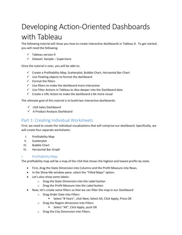
IV.button next to Text: with the three dots, and type “Profit” and “Sales” into the EditLabel window like it looks in the image.o Note: while you cannot see the labels now, you will be able to when we begin to filter ourdata in the Dashboard. This will make it easier for the user to quickly see the Departmentand Category, as well as the Profit and Sales numbers.Notice that your color scheme may have changed to Sales. If so, re-drag Profit into color and Sales intothe Size button.We now have our Bubble Chart. Rename Sheet 3 to “Bubble Chart”.Your chart should look like this:Horizontal Bar GraphThe horizontal bar graph will show the Profit and Sales for Product names, categories, and customersegments. First drag Segment, Category, and Product Name into Rows in that order.Now drag Sales into ColumnsRemember, while we make be making tons of sales, we may not be making much of a profit.Let’s give the graph more color by dragging Profit into the Color button. Notice that we now have information about the Profit and Sales for each specific product name, aswell as what Segment and Category the product resides in. The Sales represents the X axis, and the Profitrepresents the color of the bar. Let’s add a Filter to the graph so that we can use this filter later.o Drag Customer Name into Filters. Select All, click Apply, and click OK.

Now rearrange the data to that it shows the Items from the Highest Sales to Lowest Sales. You cando this by hovering over the first line of the graph, and clicking the little bar icon that appears.Also drag Customer Name into LabelsWe now have our bar graph. Rename Sheet 4 to “Product Bar Graph”Your graph should look like this:Part 2: Creating Dashboard 1: Using Floating, Filters and ActionsNow that we have our individual worksheets, let’s make them into an interactive dashboard. The firstdashboard will use the Profitability Map, Scatterplot, and Bubble Chart. We will use the Product BarGraph in another dashboard that interacts with the first one.Remember the filters we used in the Profitability Map? We will use those filters and will create someActions that will make the dashboard interactive, fun, and of course, useful.I.Creating the Initial Dashboard Click the Dashboard icon at the bottom of the worksheets. Notice that we have all four of our worksheets in the top left hand corner. First, drag the Profitability map into the dashboard worksheet. Now drag the Scatterplot into the bottom half of the worksheet. You should now have theProfitability Map on the top half, and the Scatterplot on the bottom half. It should look likethe graph below.

Now we need to put the Bubble Chart somewhere. We can place it on top of another Dashboard tosave screen real estate.So, select Bubble Chart, It should be highlighted. Now under“New Objects,” select Floating (see image to the right). Thismakes the graph able to float on top of another graph within thedashboard, instead of designating its own tile to the graph.After you’ve selected “Floating”, drag the Bubble Chart ontop of the Profitability Map, to the right of the South Eastern states. There is some extra whitespace there.Now we really don’t need the Titles for any of the graphs. If you select the graphs in thedashboards, a gray box appears, with a down arrowSelect each graph individually. Once the gray box appears, click the down arrow for each graphand unselect “Title.”Your dashboard should now look something like this:

II.Adding Filters Now that we have an initial dashboard, let’s make it a bit more interactive by using Filters. Filters also you to manipulate and slice the data by common attributes. In our case, we addedthe Year, Region, and City. First, let’s add this to our Profitability Map on the Dashboard. Remember the gray down arrow? Select the Profitability Map in the Dashboard, click the downarrow, go to Quick Filters, and select Year of Order Date. Do this once again, and Select Region, and City. Notice that the Filters appear on the Right sideof the Dashboard. Let’s start with the Year of Order Date Filter by making it a little bit more user-friendly. Howabout a slide option? Select the Year of Order Date Filter. The gray box will appear again. Clickthe down arrow, and select “Single Value Slider”. Now we can slide between the years. Now let’s drag the Year of Order date filter onto the Dashboard itself so that it is more easilyseen. Click the down arrow, and Select “Floating”. This will allow us to drag the filter on top ofthe dashboard, just as we did with the Bubble Chart. Ok, time to drag the filter. Where should we put it? There is some white space to the left of themap. Let’s put it there. Drag the Year of Order Date Filter to the left of California. Resize it so itfits nicely onto the graph. Let’s reformat the filter some. We don’t really need the title of the filter, and don’t need thebuttons either. Using the down arrow, unselect the Show Title option. Also, click the downarrow button, select Customize, and unselect “Show Buttons.” Now do the same with Region and City. Region:

III.ooCity:ooFormat the Region filter as a Single Value (Dropdown)Select Floating and Drag the filter under the Year filter on the Profitability MapFormat the City filter as Single Value (Dropdown)Also, click the down arrow and select Only Relevant Values. This makes sure that when youfilter something by region or State, etc., it only shows the cities that are relevant to thatregion, state, etc.o Drag the City filter under RegionYour Dashboard should now look like this:Applying Filters to All Worksheets IV.Now let’s play around with the filter(s). Notice that they are only filtering the Profitability Map. Let’smake them filter all of the worksheets, not just the map.Using the down button on each filter, select Apply to Worksheets, and select All Using This DataSource. Do this for the Year, Region, and City filters.Now notice when you filter the data, the Scatterplot and Bubble Chart change.Adding Actions to Filters Now, we also want to make the dashboard even more interactive by having the ability toselect one of the individual states, and having that filter the data as well. Notice right now, ifyou select a state on the dashboard, the Scatterplot and the Bubble Chart do not change. Forexample, select Washington. To make the other graphs change, we need to create an Action.

To do so, click on the Dashboard tab in the toolbar and select Actions.Actions allow you to create specific actions for different aspects of your dashboards to makethem more interactive. We will create an action that allows us to select a state to filter ourworksheets.In the Actions window, click Add Action and Select Filter.Rename the Filter1 Action to “State Selection.”Under “Source Sheets,” make sure to only check theProfitability Map. Remember, we want to use themap to filter the rest of the worksheets by ourselection (i.e., choosing a state).Under Run action on, we need to click “Select.” This isthe action itself. So choose “Select” because we wantto select the state, and filter the rest of the data byour selected action.We also want to have the data filter when a singlestate is selected, so we have to select “Run on singleselect only.”Under Target Sheets, leave all of them checked. Thisallows us to filter all of the worksheets in theDashboard by our single state selection.Under Target Filters, select All Fields.Click Ok, and OK again.Now when you select a single state in yourProfitability Map, you will notice that theScatterplot and the Bubble Chart change. Forexample, if I select Oregon, the Dashboard shouldlook like this: