Transcription
Information, Physics and ComputationMarc MézardLaboratoire de Physique Théorique et Modèles Statistiques,CNRS and Université Paris SudAndrea MontanariDepartments of Electrical Engineering and Statistics,Stanford University
PrefaceThe following are a few chapters from the book “Information, Physics and Computation” by M. Mézard and Andrea Montanari, collected here for the course given byMarc Mézard at the summer school in Peyresq, July 2008. The book is scheduledfor the end of 2008. Please don’t circulate the present preliminary version, and don’thesitate to signal us any misprint or error!The book itself is structured in five large parts, focusing on topics of increasingcomplexity. Each part typically contains three chapters presenting some core topicsin each of the disciplines: information theory, statistical physics, and combinatorialoptimization. The topics in each part have a common mathematical structure, whichis developed in additional chapters serving as bridges. Part A (chapters 1-4) contains introductory chapters to each of the three disciplines and some common probabilistic tools. Part B (chapters 5-8) deals with problems in which independence plays an important role: random energy model, random code ensemble, and number partitioning.Thanks to independence of random variables, classical techniques can be successfully to these problems. It ends up with a description of the replica method. Part C (chapters 9-13) describes ensembles of problems on graphs: satisfiability,low density parity check codes, and spin glasses. Factor graphs and statisticalinference provide a common language. Part D (chapters 14-17) explains belief propagation and the related ‘replica symmetric’ cavity method. These can be thought as approaches to study systems ofcorrelated random variables on large graphs. It shows the success of this approachon three problems: decoding, assignment, and ferromagnets. Part E (chapters 18-22) is dedicated to the proliferation of pure states and ‘replicasymmetry breaking.’ It starts with the simpler problem of random linear equationswith Boolean variables, then develops the general approach and applies it tosatisfiability and coding. The final chapter reviews open problems.‘‘Info Phys Comp’’ Draft: 22 July 2008 -- ‘‘Info Phys Comp
‘‘Info Phys Comp’’ Draft: 22 July 2008 -- ‘‘Info Phys Comp
Contents1Introduction to Information Theory1.1 Random variables1.2 Entropy1.3 Sequences of random variables and entropy rate1.4 Correlated variables and mutual information1.5 Data compression1.6 Data transmissionNotes113681014202Statistical physics and probability theory2.1 The Boltzmann distribution2.2 Thermodynamic potentials2.3 The fluctuation dissipation relations2.4 The thermodynamic limit2.5 Ferromagnets and Ising models2.6 The Ising spin glassNotes21222731323543453Introduction to combinatorial optimization3.1 A first example: minimum spanning tree3.2 General definitions3.3 More examples3.4 Elements of the theory of computational complexity3.5 Optimization and statistical physics3.6 Optimization and codingNotes46475050535960615The Random Energy Model5.1 Definition of the model5.2 Thermodynamics of the REM5.3 The condensation phenomenon5.4 A comment on quenched and annealed averages5.5 The random subcube modelNotes636364697173756Random Code Ensemble6.1 Code ensembles6.2 Geometry of the Random Code Ensemble6.3 Communicating over the Binary Symmetric Channel6.4 Error-free communication with random codes7676798189‘‘Info Phys Comp’’ Draft: 22 July 2008 -- ‘‘Info Phys Comp
viiiContents6.5 Geometry again: sphere packing6.6 Other random codes6.7 A remark on coding theory and disordered systemsNotes9Factor graphs and graph ensembles9.1 Factor graphs9.2 Ensembles of factor graphs: definitions9.3 Random factor graphs: basic properties9.4 Random factor graphs: The giant component9.5 The locally tree-like structure of random graphsNotes92959697999910610811311712010 Satisfiability10.1 The satisfiability problem10.2 Algorithms10.3 Random K-satisfiability ensembles10.4 Random 2-SAT10.5 Phase transition in random K( 3)-SATNotes12212212413113313414211 Low-Density Parity-Check Codes11.1 Definitions11.2 Geometry of the codebook11.3 LDPC codes for the binary symmetric channel11.4 A simple decoder: bit flippingNotes14414514715616116412 Spin glasses12.1 Spin glasses and factor graphs12.2 Spin glasses: Constraints and frustration12.3 What is a glass phase?12.4 An example: the phase diagram of the SK modelNotes16616617017518719014 Belief propagation14.1 Two examples14.2 Belief Propagation on tree graphs14.3 Optimization: max-product and min-sum14.4 Loopy BP14.5 General message passing algorithms14.6 Probabilistic analysisNotes19219319720621121821922715 Decoding with belief propagation15.1 BP decoding: the algorithm15.2 Analysis: density evolution15.3 BP decoding of the erasure channel229229231244‘‘Info Phys Comp’’ Draft: 22 July 2008 -- ‘‘Info Phys Comp
Contents15.4 Bethe free-energy and MAP decodingNotesix249254Appendix A Symbols and notationsA.1 Equivalence relationsA.2 Orders of growthA.3 Combinatorics and probabilityA.4 Summary of mathematical notationsA.5 Information theoryA.6 Factor graphsA.7 Cavity and Message Info Phys Comp’’ Draft: 22 July 2008 -- ‘‘Info Phys Comp
1Introduction to Information TheoryThis chapter introduces some of the basic concepts of information theory, as well asthe definitions and notations of probability theory that will be used throughout thebook. The notion of entropy, which is fundamental to the whole topic of this book,is introduced here. We also present the main questions of information theory, datacompression and error correction, and state Shannon’s theorems.Sec. 1.1 introduces basic notations in probability. The notion of entropy, and theentropy rate of a sequence , are discussed in Sec. 1.2 and 1.3. A very important conceptin information theory is the mutual information of correlated random variables, is isintroduced in 1.4. Then we move to the two main aspects of the theory, the compressionof data in Sec. 1.5 and the transmission in Sec. 1.6.1.1Random variablesThe main object of this book will be the behavior of large sets of discrete randomvariables . A discrete random variable X is completely defined1 by the set of valuesit can take, X , which we assume to be a finite set, and its probability distribution{pX (x)}x X . The value pX (x) is the probability that the random variable X takes thevalue x. The probability distribution pX : X [0, 1] is a non-negative function thatsatisfies the normalization condition:XpX (x) 1 .(1.1)x XWe shall denote by P(A) the probability of an event A X , so that pX (x) P(X x). To lighten notations, when there is no ambiguity, we use p(x) to denote pX (x).If f (X) is a real valued function of the random variable X, the expectation valueof f (X), which we shall also call the average of f , is denoted by:XEf pX (x)f (x) .(1.2)x XWhile our main focus will be on random variables taking values in finite spaces,we shall sometimes make use of continuous random variables taking values inRd or in some smooth finite-dimensional manifold. The probability measure for an‘infinitesimal element’ dx will be denoted by dpX (x). Each time pX admits a density1 In probabilistic jargon (which we shall avoid hereafter), we take the probability spaceP(X , P(X ), pX ) where P(X ) is the σ-field of the parts of X and pX x X pX (x) δx .‘‘Info Phys Comp’’ Draft: 22 July 2008 -- ‘‘Info Phys Comp
2Introduction to Information Theory(with respect to the Lebesgue measure), we shall use the notation pX (x) for the valueof this density at the point x. The total probability P(X A) that the variable Xtakes value in some (measurable) set A X is given by the integral:P(X A) ZdpX (x) x AZI(x A) dpX (x) ,(1.3)where the second form uses the indicator function I(s) of a logical statement s,whichis defined to be equal to 1 if the statement s is true, and equal to 0 if the statementis false.The expectation value E f (X) and the variance Var f (X) of a real valued functionf (x) are given by:E f (X) Zf (x) dpX (x) ;Var f (X) E{f (X)2 } {E f (X)}2(1.4)Sometimes we may write EX f (X) for specifying the variable to be integrated over.We shall often use the shorthand pdf for the probability density function pX (x).Example 1.1 A fair dice with M faces has X {1, 2, . . . , M } and p(i) 1/M forall i {1, . . . , M }. The average of x is E X (1 · · · M )/M (M 1)/2.Example 1.2 Gaussian variable: a continuous variable X R has a Gaussian distribution of mean m and variance σ 2 if its probability density is [x m]21.(1.5)exp p(x) 2σ 22πσOne has EX m and E(X m)2 σ 2 .Appendix A contains definitions and notations for the random variables that weshall encounter most frequentlyThe notations of this chapter mainly deal with discrete variables. Most of theexpressionscan be transposed to the case of continuous variables by replacing sumsPbyintegralsand interpreting p(x) as a probability density.xExercise 1.1 Jensen’s inequality. Let X be a random variable taking value in a set X Rand f a convex function (i.e. a function such that x, y and α [0, 1]: f (αx (1 α)y) αf (x) (1 α)f (y). ThenEf (X) f (EX) .(1.6)Supposing for simplicity that X is a finite set with X n, prove this equality by recursionon n.‘‘Info Phys Comp’’ Draft: 22 July 2008 -- ‘‘Info Phys Comp
Entropy1.23EntropyThe entropy HX of a discrete random variable X with probability distribution p(x)is defined as X1p(x) log2 p(x) E log2HX ,(1.7)p(X)x Xwhere we define by continuity 0 log2 0 0. We shall also use the notation H(p) whenever we want to stress the dependence of the entropy upon the probability distributionof X.In this Chapter we use the logarithm to the base 2, which is well adapted to digitalcommunication, and the entropy is then expressed in bits. In other contexts, andin particular in statistical physics, one rather uses the natural logarithm (with basee 2.7182818). It is sometimes said that, in this case, entropy is measured in nats.In fact, the two definitions differ by a global multiplicative constant, which amountsto a change of units. When there is no ambiguity we use H instead of HX .Intuitively, the entropy HX is a measure of the uncertainty of the random variableX. One can think of it as the missing information: the larger the entropy, the less apriori information one has on the value of the random variable. It roughly coincideswith the logarithm of the number of typical values that the variable can take, as thefollowing examples show.Example 1.3 A fair coin has two values with equal probability. Its entropy is 1 bit.Example 1.4 Imagine throwing M fair coins: the number of all possible outcomesis 2M . The entropy equals M bits.Example 1.5 A fair dice with M faces has entropy log2 M .Example 1.6 Bernoulli process. A Bernoulli random variable X can take values0, 1 with probabilities p(0) q, p(1) 1 q. Its entropy isHX q log2 q (1 q) log2 (1 q) ,(1.8)it is plotted as a function of q in Fig.1.1. This entropy vanishes when q 0 or q 1because the outcome is certain, it is maximal at q 1/2 when the uncertainty onthe outcome is maximal.Since Bernoulli variables are ubiquitous, it is convenient to introduce the functionH(q) q log q (1 q) log(1 q), for their entropy.‘‘Info Phys Comp’’ Draft: 22 July 2008 -- ‘‘Info Phys Comp
4Introduction to Information Theory10.90.80.70.6H(q) 0.50.40.30.20.1000.10.20.30.40.50.60.70.80.91qFig. 1.1 The entropy H(q) of a binary variable with p(X 0) q, p(X 1) 1 q,plotted versus qExercise 1.2 An unfair dice with four faces and p(1) 1/2, p(2) 1/4, p(3) p(4) 1/8 has entropy H 7/4, smaller than the one of the corresponding fair dice.Exercise 1.3 DNA is built from a sequence of bases which are of four types, A,T,G,C. Innatural DNA of primates, the four bases have nearly the same frequency, and the entropy perbase, if one makes the simplifying assumptions of independence of the various bases, is H log2 (1/4) 2. In some genus of bacteria, one can have big differences in concentrations:p(G) p(C) 0.38, p(A) p(T ) 0.12, giving a smaller entropy H 1.79.Exercise 1.4 In some intuitive way, the entropy of a random variable is related to the‘risk’ or ‘surprise’ which are associated to it. Let us see how these notions can be mademore precise.Consider a gambler who bets on a sequence of Bernoulli random variables Xt {0, 1},t {0, 1, 2, . . . } with mean EXt p. Imagine he knows the distribution of the Xt ’s and, attime t, he bets a fraction w(1) p of his money on 1 and a fraction w(0) (1 p) on 0.He looses whatever is put on the wrong number, while he doubles whatever has been puton the right one. Define the average doubling rate of his wealth at time t as1Wt E log2t(tYt′ 1)2w(Xt′ ).(1.9)It is easy to prove that the expected doubling rate EWt is related to the entropy of Xt :EWt 1 H(p). In other words, it is easier to make money out of predictable events.‘‘Info Phys Comp’’ Draft: 22 July 2008 -- ‘‘Info Phys Comp
Entropy5Another notion that is directly related to entropy is the Kullback-Leibler (KL)divergence between two probability distributions p(x) and q(x) over the same finitespace X . This is defined as:D(q p) Xx Xq(x) logq(x)p(x)(1.10)where we adopt the conventions 0 log 0 0, 0 log(0/0) 0. It is easy to show that: (i)D(q p) is convex in q(x); (ii) D(q p) 0; (iii) D(q p) 0 unless q(x) p(x). The lasttwo properties derive from the concavity of the logarithm (i.e. the fact that the function log x is convex) and Jensen’s inequality (1.6): if E denotes expectation with respectto the distribution q(x), then D(q p) E log[p(x)/q(x)] log E[p(x)/q(x)] 0. TheKL divergence D(q p) thus looks like a distance between the probability distributionsq and p, although it is not symmetric.The importance of the entropy, and its use as a measure of information, derivesfrom the following properties:1. HX 0.2. HX 0 if and only if the random variable X is certain, which means that Xtakes one value with probability one.3. Among all probability distributions on a set X with M elements, H is maximumwhen all events x are equiprobable, with p(x) 1/M . The entropy is then HX log2 M .To prove this statement, notice that if X has M elements then the KL divergenceD(p p) between p(x) and the uniform distribution p(x) 1/M is D(p p) log2 M H(p). The statement is a direct consequence of the properties of the KLdivergence.4. If X and Y are two independent random variables, meaning that pX,Y (x, y) pX (x)pY (y), the total entropy of the pair X, Y is equal to HX HY :HX,Y XpX,Y (x, y) log2 pX,Y (x, y)x,yXpX,Y (x, y) (log2 pX (x) log2 pY (y)) HX HY(1.11)x,y5. For any pair of random variables, one has in general HX,Y HX HY , and thisresult is immediately generalizable to n variables. (The proof can be obtained byusing the positivity of KL divergence D(p1 p2 ), where p1 pX,Y and p2 pX pY ).6. Additivity for composite events. Take a finite set ofPevents X , and decompose itinto X X1 X2 , where X1 X2 . Call q1 x X1 p(x) the probability ofX1 , and q2 the probability of X2 . For each x X1 , define as usual the conditionalprobability of x, given that x X1 , by r1 (x) p(x)/q1 and define similarly r2 (x)as the conditional probability of x, given that x X2 . ThenP the total entropycan be written as the sum of two contributions HX x X p(x) log2 p(x) e r), where:H(q) H(q,‘‘Info Phys Comp’’ Draft: 22 July 2008 -- ‘‘Info Phys Comp
6Introduction to Information TheoryH(q) q1 log2 q1 q2 log2 q2XXe r) q1H(q,r1 (x) log2 r1 (x) q2r2 (x) log2 r2 (x)x X1(1.12)(1.13)x X1The proof is straightforward by substituting the laws r1 and r2 by their definitions.This property is interpreted as the fact that the average information associated tothe choice of an event x is additive, being the sum of the relative information H(q)associated to a choice of subset, and the information H(r) associated to the choiceof the event inside the subsets (weighted by the probability of the subsets). It is themain property of the entropy, which justifies its use as a measure of information.In fact, this is a simple example of the so called chain rule for conditional entropy,which will be further illustrated in Sec. 1.4.Conversely, these properties together with appropriate hypotheses of continuityand monotonicity can be used to define axiomatically the entropy.1.3Sequences of random variables and entropy rateIn many situations of interest one deals with a random process which generates sequences of random variables {Xt }t N , each of them taking values in the same finitespace X . We denote by PN (x1 , . . . , xN ) the joint probability distribution of the first Nvariables. If A {1, . . . , N } is a subset of indices, we shall denote by A its complementA {1, . . . , N } \ A and use the notations xA {xi , i A} and xA {xi , i A}(the set subscript will be dropped whenever clear from the context). The marginaldistribution of the variables in A is obtained by summing PN on the variables in A:PA (xA ) XPN (x1 , . . . , xN ) .(1.14)xAExample 1.7 The simplest case is when the Xt ’s are independent. This means thatPN (x1 , . . . , xN ) p1 (x1 )p2 (x2 ) . . . pN (xN ). If all the distributions pi are identical,equal to p, the variables are independent identically distributed, which will beabbreviated as i.i.d. The joint distribution isPN (x1 , . . . , xN ) NYp(xi ) .(1.15)t 1‘‘Info Phys Comp’’ Draft: 22 July 2008 -- ‘‘Info Phys Comp
Sequences of random variables and entropy rate7Example 1.8 The sequence {Xt }t N is said to be a Markov chain ifPN (x1 , . . . , xN ) p1 (x1 )N 1Yt 1w(xt xt 1 ) .(1.16)Here {p1 (x)}x X is called the initial state, and {w(x y)}x,y X are the transitionprobabilities of the chain. The transition probabilities must be non-negative andnormalized:Xw(x y) 1 ,for any x X .(1.17)y XWhen we have a sequence of random variables generated by a certain process, it isintuitively clear that the entropy grows with the number N of variables. This intuitionsuggests to define the entropy rate of a sequence xN {Xt }t N ashX lim HX N /N ,N (1.18)if the limit exists. The following examples should convince the reader that the abovedefinition is meaningful.Example 1.9 If the Xt ’s are i.i.d. random variables with distribution {p(x)}x X ,the additivity of entropy impliesXhX H(p) p(x) log p(x) .(1.19)x X‘‘Info Phys Comp’’ Draft: 22 July 2008 -- ‘‘Info Phys Comp
8Introduction to Information TheoryExample 1.10 Let {Xt }t N be a Markov chain with initial state {p1 (x)}x X andtransition probabilities {w(x y)}x,y X . Call {pt (x)}x X the marginal distributionof Xt and assume the following limit to exist independently of the initial condition:p (x) lim pt (x) .t (1.20)As we shall see in chapter ?, this turns indeed to be true under quite mild hypotheseson the transition probabilities {w(x y)}x,y X . Then it is easy to show thatXhX p (x) w(x y) log w(x y) .(1.21)x,y XIf you imagine for instance that a text in English is generated by picking lettersrandomly in the alphabet X , with empirically determined transition probabilitiesw(x y), then Eq. (1.21) gives a rough estimate of the entropy of English.A more realistic model is obtained using a Markov chain with memory. Thismeans that each new letter xt 1 depends on the past through the value of the kprevious letters xt , xt 1 , . . . , xt k 1 . Its conditional distribution is given by the transition probabilities w(xt , xt 1 , . . . , xt k 1 xt 1 ). Computing the correspondingentropy rate is easy. For k 4 one gets an entropy of 2.8 bits per letter, much smallerthan the trivial upper bound log2 27 (there are 26 letters, plus the space symbols),but many words so generated are still not correct English words. Better estimates ofthe entropy of English, through guessing experiments, give a number around 1.3.1.4Correlated variables and mutual informationGiven two random variables X and Y , taking values in X and Y, we denote theirjoint probability distribution as pX,Y (x, y), which is abbreviated as p(x, y), and theconditional probability distribution for the variable y given x as pY X (y x), abbreviatedas p(y x). The reader should be familiar with Bayes classical theorem:p(y x) p(x, y)/p(x) .(1.22)When the random variables X and Y are independent, p(y x) is x-independent.When the variables are dependent, it is interesting to have a measure on their degree ofdependence: how much information does one obtain on the value of y if one knows x?The notions of conditional entropy and mutual information will answer this question.Let us define the conditional entropy HY X as the entropy of the law p(y x),averaged over x:XXHY X p(x)p(y x) log2 p(y x) .(1.23)x Xy YPThe joint entropy HX,Y x X ,y Y p(x, y) log2 p(x, y) of the pair of variables x, ycan be written as the entropy of x plus the conditional entropy of y given x, an identityknown as the chain rule:HX,Y HX HY X .(1.24)‘‘Info Phys Comp’’ Draft: 22 July 2008 -- ‘‘Info Phys Comp
Correlated variables and mutual information9In the simple case where the two variables are independent, HY X HY , andHX,Y HX HY . One way to measure the correlation of the two variables is themutual information IX,Y which is defined as:Xp(x, y).p(x)p(y)(1.25)IX,Y HY HY X HX HX Y .(1.26)IX,Y p(x, y) log2x X ,y YIt is related to the conditional entropies by:This shows that the mutual information IX,Y measures the reduction in the uncertaintyof x due to the knowledge of y, and is symmetric in x, y.Proposition 1.11 IX,Y 0. Moreover IX,Y 0 if and only if X and Y are independent variables.Proof: Write IX,Y Ex,y log2 p(x)p(y)p(x,y) . Consider the random variable u (x, y)with probability distribution p(x, y). As the function log( · ) is convex, one can applyJensen’s inequality (1.6). This gives the result IX,Y 0 Exercise 1.5 A large group of friends plays the following game (telephone without cables). The guy number zero chooses a number X0 {0, 1} with equal probability andcommunicates it to the first one without letting the others hear, and so on. The first guycommunicates the number to the second one, without letting anyone else hear. Call Xnthe number communicated from the n-th to the (n 1)-th guy. Assume that, at each stepa guy gets confused and communicates the wrong number with probability p. How muchinformation does the n-th person have about the choice of the first one?We can quantify this information through IX0 ,Xn In . Show that In 1 H(pn ) withpn given by 1 2pn (1 2p)n . In particular, as n In (1 2p)2n ˆ1 O((1 2p)2n ) .2 log 2(1.27)The ‘knowledge’ about the original choice decreases exponentially along the chain.mutual information gets degraded when data is transmitted or processed. This isquantified by:Proposition 1.12 (Data processing inequality). Consider a Markov chain X Y Z (so that the joint probability of the three variables can be written as p1 (x)w2 (x y)w3 (y z)). Then: IX,Z IX,Y . In particular, if we apply this result to the casewhere Z is a function of Y , Z f (Y ), we find that applying f degrades the information: IX,f (Y ) IX,Y .Proof: Let us introduce, in general, the mutual information of two variables conditioned to a third one: IX,Y Z HX Z HX (Y Z) . The mutual information betweena variable X and a pair of variables (Y Z) can be decomposed using the following‘‘Info Phys Comp’’ Draft: 22 July 2008 -- ‘‘Info Phys Comp
10Introduction to Information Theorychain rule : IX,(Y Z) IX,Z IX,Y Z IX,Y IX,Z Y . If we have a Markov chainX Y Z, X and Z are independent when one conditions on the value of Y ,therefore IX,Z Y 0. The result follows from the fact that IX,Y Z 0. conditional entropy also gives a bound on the possibility to guess a variable. Suppose you want to guess the value of the random variable X, but you observe onlythe random variable Y (which can be thought as a noisy version of X). From Y , youb g(Y ) which is your estimate for X. What is the probabilitycompute a function XPe that you guessed incorrectly? Intuitively, if X and Y are strongly correlated onecan expect that Pe is small, while it increases for less correlated variables. This isquantified by:Proposition 1.13 (Fano’s inequality). Consider a random variable X taking valuesb where Xb g(Y ) is an estimatein the alphabet X , and the Markov chain X Y Xbfor the value of X. Define as Pe P(X 6 X) the probability to make a wrong guess.It is bounded below as follows:H(Pe ) Pe log2 ( X 1) H(X Y ) .(1.28)b 6 X) equal to 0 if Xb X, and toProof: Define the random variable E I(X1 otherwise, and decompose the conditional entropy HX,E Y using the chain rule,in two ways: HX,E Y HX Y HE X,Y HE Y HX E,Y . Then notice that: (i)HE X,Y 0 (because E is a function of X and Y ); (ii) HE Y HE H(Pe ); (iii)HX E,Y (1 Pe )HX E 0,Y Pe HX E 1,Y Pe HX E 1,Y Pe log2 ( X 1). Exercise 1.6 Suppose that X can take k values, and its distribution is p(1) 1 p,pfor x 2. If X and Y are independent, what is the value of the right hand sidep(x) k 1p, what is the best guess one can make onof Fano’s inequality? Assuming that 1 p k 1the value of X? What is the probability of error? Show that Fano’s inequality holds as anequality in this case.1.5Data compressionImagine an information source which generates a sequence of symbols X {X1 , . . . , XN }taking values in a finite alphabet X . Let us assume a probabilistic model for the source,meaning that the Xi ’s are random variables. We want to store the information contained in a given realization x {x1 . . . xN } of the source in the most compact way.This is the basic problem of source coding. Apart from being an issue of utmostpractical interest, it is a very instructive subject. It allows in fact to formalize in aconcrete fashion the intuitions of ‘information’ and ‘uncertainty’ which are associatedwith the definition of entropy. Since entropy will play a crucial role throughout thebook, we present here a little detour into source coding.‘‘Info Phys Comp’’ Draft: 22 July 2008 -- ‘‘Info Phys Comp
Data compression1.5.111CodewordsWe first need to formalize what is meant by “storing the information”. We define asource code for the random variable X to be a mapping w which associates to anypossible information sequence in X N a string in a reference alphabet which we shallassume to be {0, 1}:w : X N {0, 1} x 7 w(x) .(1.29)Here we used the convention of denoting by {0, 1} the set of binary strings of arbitrarylength. Any binary string which is in the image of w is called a codeword.Often the sequence of symbols X1 . . . XN is a part of a longer stream. The compression of this stream is realized in three steps. First the stream is broken into blocksof length N . Then each block is encoded separately using w. Finally the codewordsare glued to form a new (hopefully more compact) stream. If the original stream consisted in the blocks x(1) , x(2) , . . . , x(r) , the output of the encoding process will be theconcatenation of w(x(1) ), . . . , w(x(r) ). In general there is more than one way of parsingthis concatenation into codewords, which may cause troubles when one wants to recover the compressed data. We shall therefore require the code w to be such that anyconcatenation of codewords can be parsed unambiguously. The mappings w satisfyingthis property are called uniquely decodable codes.Unique decodability is surely satisfied if for any x, x′ X N , w(x) is not a prefix ofw(x′ ) (see Fig. 1.2). In such a case the code is said to be instantaneous. Hereafter weshall focus on instantaneous codes, since they are both practical and slightly simplerto analyze.Now that we precised how to store information, namely using a source code, it isuseful to introduce some figure of merit for source codes. If lw (x) is the length of thestring w(x), the average length of the code is:L(w) Xp(x) lw (x) .(1.30)x X N‘‘Info Phys Comp’’ Draft: 22 July 2008 -- ‘‘Info Phys Comp
12Introduction to Information Theory1001100111000010100101101Fig. 1.2 An instantaneous source code: each codeword is assigned to a node in a binarytree in such a way that no one among them is the ancestor of another one. Here the fourcodewords are framed.Example 1.14 Take N 1 and consider a random variable X which takes valuesin X {1, 2, . . . , 8} with probabilities p(1) 1/2, p(2) 1/4, p(3) 1/8, p(4) 1/16, p(5) 1/32, p(6) 1/64, p(7) 1/128, p(8) 1/128. Consider the twocodes w1 and w2 defined by the table belowx p(x)1 1/22 1/43 1/84 1/165 1/326 1/647 1/1288 1/128w1 (x) w2 (x)000000110010110011111010011110101 111110110 1111110111 11111110(1.31)These two codes are instantaneous. For instance looking at the code w2 , the encodedstring 10001101110010 can be parsed in only one way since each symbol 0 ends acodeword . It thus corresponds to the sequence x1 2, x2 1, x3 1, x4 3, x5 4, x6 1, x7 2. The average length of code w1 is L(w1 ) 3, the average lengthof code w2 is L(w2 ) 247/128. Notice that w2 achieves a shorter average lengthbecause it assigns the shortest codeword (namely 0) to the most probable symbol(i.e. x 1).Example 1.15 A useful graphical representation of a source code is obtained bydrawing a binary tree and associating each codeword to the corresponding node inthe tree. In Fig. 1.2 we represent in this way a source code with X N 4. It isquite easy to recognize that the code is indeed instantaneous. The codewords, whichare framed, are such that no codeword is the ancestor of any other codeword in thetree. Given a sequence of codewords, parsing is immediate. For instance the sequen
10.2 Algorithms 124 10.3 Random K-satisfiability ensembles 131 10.4 Random 2-SAT 133 10.5 Phase transition in random K( 3)-SAT 134 Notes 142 11 Low-Density Parity-Check Codes 144 11.1 Definitions 145 11.2 Geometry of the codebook 147 11.3 LDPC codes for the binary symmetric channel 156 11.4 A simple decoder: bit flipping 161 Notes 164 12 .