Transcription
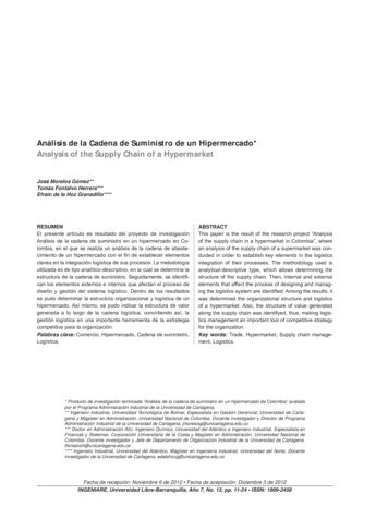
Measuring the Performance of Single Image Depth Estimation MethodsCesar Cadena, Yasir Latif, and Ian D. ReidAbstract— We consider the question of benchmarking theperformance of methods used for estimating the depth of a scenefrom a single image. We describe various measures that havebeen used in the past, discuss their limitations and demonstratethat each is deficient in one or more ways. We propose a newmeasure of performance for depth estimation that overcomesthese deficiencies, and has a number of desirable properties. Weshow that in various cases of interest the new measure enablesvisualisation of the performance of a method that is otherwiseobfuscated by existing metrics. Our proposed method is capableof illuminating the relative performance of different algorithmson different kinds of data, such as the difference in efficacyof a method when estimating the depth of the ground planeversus estimating the depth of other generic scene structure. Weshowcase the method by comparing a number of existing singleview methods against each other and against more traditionaldepth estimation methods such as binocular stereo.I. I NTRODUCTIONSingle image depth estimation methods try to predict the3D structure of a scene (i.e. the depth at each point in thescene) from a single photometric view, thus recovering thedepth information that is lost during the imaging process.Inspired in part by the ability of humans to perform this task(albeit usually qualitatively), single-view depth estimationhas become an active area within the computer vision community, with various methods proposed recently, including[1, 3, 4, 7, 9, 10, 11, 13]. To evaluate and compare the efficacy of these approaches, various metrics and methods havebeen proposed. However, as we show in this paper, each ofthese measures is deficient in one or more ways. To addressthis issue we propose a new measure of performance fordepth estimation that has a number of desirable properties.For most tasks, performance of a method to solve the taskis measured by comparing the output of the method againstsome known ground truth. In our case, we are interested indepth estimation, and the “ground truth” here is typically asingle depth image, normally acquired by a depth camera.Most existing metrics for benchmarking single-view depthestimation aim to capture, for each pixel in the predictedimage, the closeness of the prediction to the correspondingpixel in the ground truth; i.e. they operate in the image space.A number of such metrics have been reported for imagespace comparisons, and we give an overview in SectionCesar Cadena is with the Autonomous Systems Lab at ETH Zurich,Leonhardstrasse 21, 8092, Zurich, Switzerland. cesarc@ethz.chYasir Latif and Ian D. Reid are with the Department of ComputerScience, at the University of Adelaide, Adelaide, SA 5005, Australia.{yasir.latif, ian.reid} @adelaide.edu.auWe are extremely grateful to the Australian Research Council for fundingthis research through project DP130104413, the ARC Centre of Excellencefor Robotic Vision C E140100016, and through a Laureate FellowshipFL130100102 to IDR.Fig. 1: RGB image and the corresponding ground truth depthobtained using a depth camera taken from the NYU-V2 dataset.II. An issue with these metrics is that they assume thatthe estimated and ground truth depth images have the sameresolution, which is often not the case in practice. They also,typically address the issue of missing depth estimates bycalculating the metric only over the set of pixels where boththe prediction and the ground truth have values. However, aswe will show later, problems arise in scenarios where a pixelby pixel comparison is not feasible against the full resolutionground truth especially in cases when: a) the resolution ofthe prediction does not match that of the ground truth, b) thedensity of the prediction and ground truth are not the same,or c) the coverage of the prediction is not the same as thatof the ground truth (more on coverage and density later).In this work, we advocate that comparisons should alwaysbe made against the given ground truth without up/downsampling, without recourse to in-painting (hallucination) of“ground truth”, and should adequately portray how much ofthe ground truth is explained by each method. In particular,unlike most previous comparison methods, we propose tocompare the predicted depths to ground truth in 3D-spaceinstead of the image space. Section III defines our proposedperformance measure, and shows that it is agnostic to thedifferences in resolution, density, and coverage between theground truth and the estimated depths.Using the proposed measure, in Section IV we comparethe performance of state of the art single image depthestimation methods for the NYU-V2 dataset [14]. Thisdataset comes with hand labelled semantic segmentationannotations. Then, we show how our performance measuretakes advantages of the semantic classes to give more insightsfor each estimation method. Finally in Section V, we alsoshow a comparison between classical stereo depth estimationand single image depth estimation in an outdoors settingusing the KITTI dataset [5].II. C URRENT M ETRICSGiven a predicted depth image and the correspondingground truth, with dˆp and dp denoting the estimated and
ground-truth depths respectively at pixel p, and T being thetotal number of pixels for which there exist both valid groundtruth and predicted depth, the following metrics have beenreported in literature: Absolute Relative Error [13] Linear Root Mean Square Error (RMSE) [8]s1X(dp dˆp )2T psame resolution as the ground truth. Once again, we present aperformance comparison using the traditional metrics (TableI [downscaling, then upscaling])It is interesting to observe that in Table I, the performanceat each resolution is now worse than the case in whichwe down scaled the ground truth [downscaling]. Up scalingcreates information by interpolation, which may not alwaysagree with the ground truth at that particular pixel position.The smaller the original resolution, the more we upscalethe prediction, and the more error we introduce; this isreflected in the metrics. It should be noted that the initialdepth estimation is very accurate since it is derived from thein-painted ground truth. log scale invariant RMSE (as proposed in [4])B. Density1 X dp dˆp T pdp1X(log dˆp log dp α(dˆp , dp ))2T p where α(dˆp , dp ) addresses scale alignment.Accuracy under a threshold [7]!dˆp dp, δ thmaxdp dˆpwhere th is a predefined threshold.In the following, we present various cases which highlightthe deficiencies of these metrics. In the scenarios presentedhere, the ground truth is taken from the NYU-V2 dataset[14]. We use the in-painted depth from the NYU-V2 asthe estimation of the system since it is already close to theground truth, therefore, any minor differences introduced byvarious transformations can be observed more easily.A. ResolutionSingle image depth estimation methods may predict alower resolution depth image compared to the ground truth.Traditionally, comparisons for this case are done by downsizing the ground truth to the size of the estimation. However,if we insist on keeping the ground truth unchanged, theprediction can be upsampled using an appropriate scaling.A natural question is, which is a better way of comparingthe two? Should the ground truth be scaled down or theprediction scaled up for comparison? Would the performancemetrics be different in both cases?To observe the effect of different resolutions, we use 5different sized depth estimations, each derived from the inpainted depth using nearest-neighbour down-sampling: thefull resolution, half, and down to one-sixteenth of the originalimage resolution. The results can be seen in Table I [Inpainting], where the ground truth has been down sampledto match the resolution of the predicted depth. All thepredictions have more or less the same performance basedon these metrics.Instead of down-sampling the ground truth, an alternativeapproach would be to up-sample the depth predictions using some form of interpolation. Here, we use the bilinearinterpolation to up sample all the estimations to match theSingle image depth estimation involves predicting depthfor each pixel of the input image; we refer to this as “denseestimation”. On the contrary, in robotics it is common totrack a set of sparse points while estimating their depth.We refer to that scenario as being “sparse estimation”. Inthis case, depth is not available for each pixel of the imageunder consideration but only at a set of predetermined pointswhich satisfy a certain criterion (dominant corner, gradientetc.). This scenario frequently arises in a robotics settingwhen carrying out Simultaneous Localization And Mapping(SLAM).In the following, we show how the metrics behave withrespect to the density of the points. We extract dominantcorners, FAST keypoints [12], from the image and selectthe corresponding depth from the in-painted depth as theprediction for the extracted corner. This is repeated for arange of points from 10 to 2000 (as shown in Table I[keypoints]).It can be seen from Table. I [keypoints] that these metricsdo not capture the complexity of the estimation as theyare all designed for dense estimation. Complexity in thiscase just refers to the density of the prediction – predictingthe depth for fewer points is a less complex problem thanpredicting a full dense depth image. In the case of sparseprediction, the metrics are calculated over the intersection:taking into consideration only the points that are common toboth the prediction and the ground truth. This introduces afavourable bias towards systems that predict sparse depths,but do so very accurately and in the extreme case, a singlepoint predicted extremely accurately will lead to a very goodscore on most of these metrics.C. CoverageAnother aspect of the problem is that of coverage, whichis related to density but has a slight different meaning. Adense prediction that covers the whole image is said to havefull coverage. However, prediction can be dense withoutcovering the whole image (imagine the scenario when asystem predicts depths for just planar areas in the scenesuch as ground or road). Evaluating this scenario has thesame issue as that of sparse estimation: the metrics areevaluated over the intersection and therefore do not capture
TABLE I: Results on NYU-V2 200018coverage35[%]53EstimationsMeancoarseEigen et coarseal. [4]fine fineLiu et al.[10]Eigen etmulti multial. [3]downscalingFloorFloor MeanMeanEigen etal. [4]Liu et al.[10]Eigen et al. [3]StructureStruct. MeanMeanEigen etal. [4]Liu et al.[10]Eigen et al. [3]FurnitureFurn. MeanMeanEigen etal. [4]Liu et al.[10]Eigen et al. [3]PropsProps MeanMeanEigen etal. [4]Liu et al.[10]Eigen et al. [3] coarse fine multi coarse fine multi coarse fine multi coarse fine .1430.1920.139ErrorsRMSElinear [m]log.sc.inv. 211.3e-3100.0Full Scene 90.630.19270.9Per Semantic ClassAccuracyδ 1.252 .999.9100.0100.0100.0100.0100.0100.01.253 .090.183.895.496.696.696.0the complexity of the problem. When making comparisons, asystem that does not predict at full coverage would thereforehave an unfair advantage over those that make a full denseprediction.To observe the effect of coverage on these metrics, we usecropped versions of the in-painted depth at various coveragelevels as shown in Fig. 2. The evaluation is report in TableI [coverage], where the smallest coverage has the lowestRMSE, that is, it performs better by predicting just 18%of all the depths in the ground truth.III. P ROPOSED P ERFORMANCE M EASUREWe propose to compare the predicted depth against theground truth in the 3D space instead of the image space. Fora pixel p with image coordinates up and vp and a predicteddepth dˆp , the point in 3D is given byx̂ dˆp K 1 xpwhere K contains the known camera intrinsics and xp T[up vp 1] . Similarly, for each point in the ground truth, acorresponding point x in the 3D-space can be calculated.
54.51.5413.5z [m]y [m]0.5032.5-0.52-1-2-10x [m]121.5-2-1012x [m]Fig. 3: A toy example to evaluate the accuracy of the estimation(red crosses) with respect to the ground truth (blue circles). Thecyan lines denote the closest estimated point to each ground truth3D point.Fig. 2: We evaluate the effect of three different partial coverages ofthe scene. In the figure we show one depth image with rectanglescovering the 53% (blue, solid line), 35% (red, dot-dashed line) and18% (yellow, dashed line) of the full scene.For each point xi in the ground truth, we search for thenearest point in the estimated depth and form a set of allthese nearest-neighbour distances:S {di di min xi x̂ }(1)This set has the same cardinality as the number of pixels inthe ground truth with valid depths. The objective functionminimised by the Iterative Closest Point (ICP) algorithm istypically based on a sum or robust sum over S, and so ourmeasure naturally generalises to the case where there is arigid misalignment between the ground-truth and the estimated depth (via application of ICP). In all the evaluationswe report, however, the depth esimates and ground truth arealready aligned.For a given threshold D, we look for the distances in S,that are less that D:SD {di di S di D}(2)and plot the ratio of cardinalities SD / S which representsthe fraction of ground truth that is explained by the estimation with a distance less that D. This threshold is increaseduntil all of the ground truth is explained; that is, the ratioreaches 1.Comparison using the closest point error allows forcertain nice properties: it is no longer required to havethe same resolution of the estimation and ground truthsince a closest point always exists for each point in theground truth. A visual representation of the metric, whereeach point in the ground truth is connected to its nearestneighbour can be see in Fig. 3. Moreover, now we havea systematic way of comparing estimations with differentdensities and different coverages. To illustrate, we revisitthe scenarios presented in Section II.Resolution: We first compare the performance using theproposed measure for the five down-sampled resolutionsderived from the in-painted ground truth. The results arepresented in Fig. 4a. It can been seen that under this measure,the difference in performance between various resolutions isprominent with the full resolution in-painted depth performing the best. Under older metrics, all the resolutions had moreor less the same performance. The inset in Fig. 4a shows azoom-in on the top-left corner to highlight the performanceof the curves starting very close to 1. As we expect, higherresolution estimations perform better than lower resolutions.The other case discussed in Section II is that of upsampling the estimated depth to the resolution of the groundtruth. Under the proposed performance measure, Fig. 4bshows a significant improvement for all curves. Up scaling,while introducing errors in the image space, leads to areduction in the distance to the nearest neighbour (onaverage) for each ground truth point in 3D-space. Thisleads to the gain in performance reflected here. Later on,for real single image depth prediction methods, we showthat the up scaling does not have a significant effect onthe performance measure. This is because the initial lowresolution estimation is far from the ground truth and thenthe interpolation during up sampling does not help.Density: It can be seen in Fig. 4c that by requiring that eachground truth point have a corresponding nearest-neighbourin the 3D-space, sparser predictions are ranked correctly,that is, in order of their complexity. This is true since theestimated depth has been derived from the ground truthand all the predictions for point depths are almost correct.However, methods are penalized when the points are sparseas the nearest neighbour for a ground truth lies farther away.Coverage: The results for the proposed measure are shownin Fig. 4d, which paints a more complete picture than thescalar metrics in Table I. From the perspective of the possibleexplanation of ground truth, higher coverage performs better.Finally, we show a side-by-side comparison for all thethree previous cases in Fig. 5 where we show the fullin-painted prediction, a down-sample one-sixteenth version,1000 strongest key-points, and a partial coverage scenario.It can be seen that the partial coverage behaves the worst,even though it starts off higher than other curves. The reasonbehind this is that in order to explain the full ground truthwith the partial coverage, the nearest neighbour for the
10.9111/21/41/81/160.90.80.7zoom inGT explained0.71GT explained0.80.60.980.50.960.40.60.511/16 resolution1000 00.0250.050.10.50.10.050.10.51251000.025distance [m](a) Evaluation of low resolution version of inpainted depth.111/21/41/81/160.90.80.050.10.512510distance [m]Fig. 5: Comparison between 1/16 low resolution (40x30 1200points), 1000 extracted keypoints, and a partial box of540x100 54000 points (18% coverage).zoom in0.7GT 0250.050.10.050.10.50.512510distance [m](b) Bilinear upscaling of low resolution versions of inpainteddepth. 10.90.8GT explained0.7IV. C OMPARING THE STATE OF THE ART IN I NDOORSup to 10up to 50up to 100up to 500up to 1000up to e [m](c) Keypoints.10.90.8GT explained0.70.60.50.40.53 coverage0.35 coverage0.18 coverage0.30.20.100.025ground truth point is further away than in all the other cases,leading to the slow rise of the curve. It can be said thatthe performance of the down-sampled prediction is betterthan the keypoints as the down-sampled prediction providesalmost the same amount of point (1200) but does so over aregular grid in the the 3D space (induced by the regularityof the image grid), while the keypoints are not uniformlydistributed and are defined by the structure of the scene. Theproposed method allows us to compare these different kindsof depth estimates which would not be meaningful undertraditional metrics.0.050.10.512510distance [m](d) Partial coverages.Fig. 4: Different cases evaluated in this section.Previous sections presented some toy case studies ofvarious situations in which using the proposed measure leadsto a more meaningful comparison. This section providesthe performance evaluation of some of the state-of-the-artalgorithms using the proposed method; in particular weprovide results for Eigen et al. [4] (coarse, fine), Liu et al.[10] and Eigen and Fergus [3].The system of Liu et al. [10] makes the prediction atthe same resolution as the ground truth, while the othertwo methods make depth prediction at lower resolution.For the latter, we use both the original predictions as wellas upscaled version using bilinear interpolation. Table I[Full scene evaluation] reports the comparison for all thesecombinations as well as the mean of the training data.We first consider the performance of the original (beforeupscaling) predictions where the ground truth has been scaleddown to the same resolution as the prediction. Using the oldmetrics there is a difference in ordering of performance whenwe compare the upscaled versus the original predictions.The accuracy under a threshold measure is not effected byupscaling, but in general, simple upscaling leads to a betterperformance on the other metrics, as well as permuting theorder of performance.We now turn to the evaluation on the basis of the proposedmethod, in Fig. 7. The solid lines represent the original
-2-1.5-1-1-0.5-0.5y [m]y [m]-2-1.500.500.5111.51.5-3-2-10123-3-2-1x [m]65.5554.54.51234z [m]4z [m]0x [m]65.53.53.5332.52.5221.51.511-3-2-10123-3x [m]-2-10123x [m]110.90.90.80.80.70.7eigen coarseeigen fineeigen multieigen coarse upeigen fine upeigen multi up0.60.50.4GT explainedGT explainedFig. 6: One example from the NYU-V2 test set. Left to Right: Ground truth, Inpainted Ground Truth, Liu et al. [10], Eigen et al. [4]coarse, Eigen et al. [4] fine, and Eigen and Fergus [3]. From top to bottom : Depth Image, XY-view and XZ-view of the point cloud. Thecorresponding RGB image is shown in Fig. tance [m]Fig. 7: Performance of orginal and full resolution depth estimates:eigen coarse and eigen fine [4], eigen multi [3], up indicatesupscaling to the ground truth resolutionestimates, while the dashed lines represent the upsampledversions. It can been seen that upsampling has no effect onthe order of the curves.We also present the output of these methods at a resolutionmatching the ground truth in Fig. 8. This gives an overviewof the performance for each method. For a given allowederror, we can see the percentage of the ground truth thatis associated with that distance. Additionally, the curve thatremains higher than all the rest shows that is more accurateat every given distance compared to other methods. We caninterpret this in terms of the distribution of the closest-pointdistance from the ground truth. The sharp rise in the middleindicates that the majority of distances lie in this area whichare responsible for explaining most of the ground truth.A. Break down by classesThe comparison presented so far has been over the fullscenes in the NYU-V2 dataset without taking into accountthe semantic segmentation the dataset also provides. Sinceliueigen coarse upeigen fine upeigen multi upmean0.500.0250.050.10.512510distance [m]Fig. 8: Performance of full resolution depth estimates: liu [10],eigen coarse and eigen fine [4], eigen multi [3]our proposed method is resolution, density, and coverageagnostic, we can use it to provide deeper insight into eachmethod to evaluate their performance on each individualsemantic class. The dataset provides ground truth semanticsfor categories such as Floor, Structure, Furniture, and Props.To evaluate the per class performance, we use only thepart of the ground truth with the particular class labeland compare it against the whole prediction. This allowsus to compare the semantic labels even when there is noprediction of them in the original methods. We also report thecomparison of semantics against the mean of the dataset aswell the mean over each semantic category. This allows us tohave a “look under the hood” to find out why a given methodperforms better than others. Some semantic categories suchas floor have lower complexity than others such as props,due to intra-class variations in depths.Performance for each semantic category is given in Fig. 9.Curves that remain higher than the category mean have abetter prediction of the semantic category on average forthat class label. This can been seen in the Structure subplot,
This section provides the performance evaluation ofEigen et al. [4] and Cadena et al. [2] under our proposedmeasure for an outdoors setting, specifically on the KITTIdataset [5]. Authors of [4] already provide the single imagedepth estimations and the set of frames for testing.This dataset provides 3D point clouds from a rotatingLIDAR scanner. We project the 3D information on the leftimage for each frame to obtain the ground truth depth usingthe official toolbox provided with the dataset. This projectionresults in sparse depth images covering the bottom part ofthe RGB image, see Fig. 10 left. This ground truth is usedfor all the evaluations.For comparison purposes and given that the dataset alsoprovides the right images, we compute the depth fromthe stereo pair using the basic semi-global block matchingalgorithm [6], in a setting which gives almost dense coverage.We also compute the depth of around 1000 FAST extractedkeypoints [12] in the stereo images. An example of thesedepth estimations from stereo is shown in Fig. 10 middle.With the traditional metrics, shown in Table II, the stereoestimations perform the best. Even the “dense” and “sparse”estimation seems to perform equally well. This is anotherexample of the flaws of the currently used metrics. It is clear,that the sparse stereo is giving us less information about thescene, for which should be penalized.On the other hand, our measure of performance, shownin Fig. 11, tells a better story with a coherent ordering ofthe methods. The sparse stereo performs the worst, whilea denser stereo performs in general better than single imagedepth estimation, as expected, since it provides more accurateestimations while covering the whole scene. To note, theestimations from [2] explain as much ground truth as thedense stereo method up to 15cm of error, and are betterthan [4] up to an error of 40cm.0.9Floor0.8GT explained0.7liueigen coarse upeigen fine upeigen multi upmeanFloor e [m]10.9Structure0.80.7GT explainedV. P ERFORMANCE IN O UTDOORS10.60.50.40.3liueigen coarse upeigen fine upeigen multi upmeanStructure mean0.20.100.0250.050.10.512510distance [m]10.9Furniture0.80.7GT explainedwhere most of the methods are able to do a better job thanthe category mean. On the other hand, Props and Furnitureare difficult categories for these methods. Eigen et al. [4]methods also seem to have some difficulty predicting Floordepths correctly. This novel insight comes from the ability tocompare the depths class-wise without needing the predictionof class labels from the methods being evaluated.liueigen coarse upeigen fine upeigen multi upmeanFurniture e [m]10.9Props0.8VI. D ISCUSSION AND CONCLUSIONSGT explained0.7This paper has presented a better method for performanceevaluation of single image depth estimation methods. Thepresented method is agnostic to the resolution, density andcoverage of the depth estimation and we have shown boththrough case studies and real system evaluation that theseare desirable properties. This allows a uniform comparisonwithout altering the ground truth. Further, we have shownthat it allows a deeper understanding of why a certain methodperforms better than the competition based on comparisons atthe semantic category level. Although not presented here, themeasure can be applied to methods that estimate both depthand semantics. In that case, it would capture the performanceliueigen coarse upeigen fine upeigen multi upmeanProps e [m]Fig. 9: Evaluation per semantic class on NYU-V2.
TABLE II: Results on KITTI dataset.MethoddenseStereosparseEigen et coarseal. [4] fineCadena etrgbrgb-sal. [2]ErrorsRMSElinear [m] δ 1.252 [%]96.996.186.382.279.183.31.253 [%]98.297.893.792.289.492.5Fig. 10: One example from KITTI test set. Left to Right: RGB and ground truth depth from LIDAR, dense and sparse stereo depth,Eigen et al. [4] coarse and fine estimations, and Cadena et al. estimations from rgb-only and rgb and semantics [2].10.90.8GT explained0.70.60.50.40.3dense stereosparse stereoeigen coarse upeigen fine upcadena rgbcadena rgb-s0.20.100.0250.050.10.20.512510distance [m]Fig. 11: Performance of full resolution for two stereo densities(dense and sparse), eigen coarse and eigen fine [4].of both depth as well as semantic estimates in a single unifiedway.One assumption that we make is that the estimationmethod actually tries to solve the problem rather than generating random depths over the image. To avoid those tricks itis important to always assess the estimations quantitativelyand qualitatively. As we have already noted, our method alsogeneralises to the case where the ground truth and estimateddepth are measured in different coordinate frames; in thisinstance we would first apply ICP to align the scenes, anduse the closest points found in that algorithm for our analysis.R EFERENCES[1] M. Baig, V. Jagadeesh, R. Piramuthu, A. Bhardwaj, W. Di,and N. Sundaresan. Im2depth: Scalable exemplar based depthtransfer. In Applications of Computer Vision (WACV), 2014IEEE Winter Conference on, pages 145–152, 2014.[2] C. Cadena, A. Dick, and I. Reid. Multi-modal Auto-Encodersas Joint Estimators for Robotics Scene Understanding. InProc. Robotics: Science and Systems, 2016.[3] D. Eigen and R. Fergus. Predicting depth, surface normalsand semantic labels with a common multi-scale convolutionalarchitecture. In Int. Conference on Computer Vision, 2015.[4] D. Eigen, C. Puhrsch, and R. Fergus. Depth map predictionfrom a single i
Cesar Cadena, Yasir Latif, and Ian D. Reid Abstract—We consider the question of benchmarking the performance of methods used for estimating the depth of a scene from a single image. We describe various measures that have been used in the past, discuss their limitations and demonstrate that each is deficient in one or more ways. We propose a new


![Master en DIRECCIÓN DE LOGÍSTICA, TRANSPORTE Y CADENA DE SUMINISTRO [LOC]](/img/63/folleto-loc-feb21.jpg)