Transcription
Proceedings of the 1997 IEEEInternational Conferenceon Robotics and AutomationAlbuquerque, New Mexico - April 1997Real-Time Path Planning Using Harmonic PotentialsIn Dynamic EnvironmentsHans Jacob S. Feder and Jean-Jacques E. SlotineNonlinear Systems LaboratoryMassachusetts Institute of TechnologyCambridge, MA 02139,USAfederQnsl.mit.edu, jjsQmit.eduAbstracttage of these methods is that Laplace’s equation hasto be solved numerically over the whole state space,a slow process making it extremely hard to find solutions in real-time for dynamic environments - on anL x L grid the computation time scales as L4.Two notable exceptions to the use of numerical solutions of harmonic potentials are described in[lo, 111. In [lo], analytical solutions are developedfor simple shaped objects. However, they only consider static environments and the object closest to therobot, with the drawback that the robot is not influenced by any other objects in space. Similarly, [ll]usethe panel method from computational hydrodynamicsto obtain approximate closed-form solutions over theentire space given arbitrarily shaped polygonal obstacles. It is also restricted to static environments.In this paper, we extend the harmonic potentialfield method to dynamic environments for real-timepath planning in two dimensions. We also introduceanalytical solutions for multiple moving obstacles. Insection 2 we detail the analogy between fluid flow andpath planning in two dimensions. We also introduceseveral methods for defining objects in an analyticalform, and a new method for defining the goal positionof the robot. In section 3, the approach is extendedto dynamic environments. Section 4 offers concludingremarks.Motivated by fluid analogies, artificial harmonic potentials can eliminate local m i n i m a problems in robotpath planning. I n this paper, simple analytical solutions t o planar harmonic potentials are derived using tools f r o m fluid mechanics, and are applied t otwo-dimensional planning among multiple moving obstacles. These closed-form solutions enable real-timecomputation to be readily achieved.1 IntroductionThis paper develops fast algorithms for twodimensional path planning, where the task is to finda trajectory which will bring a mobile robot from aninitial position xi,to a final position xf while avoidingmoving obstacles.Robot path planning has been studied extensively,and can use local or global computations. Combination of local and global algorithms have also been suggested, where a local method is assisted by a globalplanner when needed (that is, when the robot getsstuck) as in [l],or paths from all points in space tothe goal are defined by some potential field method[2, 31. In the potential field methods, the position andshape of all obstacles in a given region is assumed tobe known and the potential function is constructed using this information. Thus, only local calculations ateach point in space are required for the robot to findthe direction it should move in. However, potentialfield methods often have the drawback that a robotcould get stuck in local minima [2, 4, 51. This problem may be solved by forcing local potential extremato lie on the boundaries of obstacles through the useof harmonic potentials, that is, of functions 4 satisfying Laplace’s equation, V24 0, often motivated by afluid or electrostatic analogy [6, 7, 8,9]. The disadvan-0-7803-3612-7-4/97 5.00 0 1997 IEEE2The Fluid AnalogyHarmonic potentials have the great advantage thatthey achieve their extremum only on the boundaryof objects. Thus no local minima will occur in theadmissible configuration space, and a path generatedby following a steepest gradient descent is guaranteedto reach the goal without hitting any objects in thedomain, if the goal is reachable. This property of harmonic potentials is the extremum property [12]. Such874
a path is in fluid mechanics termed a streamline, anddefines the path of a fluid particle.’ In using harmonicpotentials in two-dimensional path planning it is useful to draw the analog to invicid incompressible irrotational fluid flow, termed potential flow, and therebyuse different powerful tools and properties from hydrodynamics [6, 11, 12, 131 and intuition. Let the fluidvelocity at x be U(x). The assumption that the flowis irrotational states that the vorticity vanishes, thatis:V x U O H U V (x),fluid dynamics, it is convenient to work with complex potentials, rather than just the velocity potentialin order to utilize the properties of conformal mapping of complex variables for two-dimensional problems. The complex potential consist of the velocitypotential (x), as defined above, and a function calledthe stream function (x), which is constant on a pathof a fluid particle, that is, on a streamline.2 The complex potential is defined asw Z (1)where (x) is a velocity potential. Since the fluid isassumed to be incompressible, the continuity equationcan be written:v.u o. f(z),where i 2 -1.The velocity field, U [Ueither , II, or w byz s i y ;U](5)can be found from(2)Combining equation (1) and (2) we arrive at theLaplace equation for the velocity potential:V2 0 .(3)We here outline the four major methods to definevarious potential flows: simple flows, use of specifictheorems, conformal mapping and a panel method.We here use U to represent a velocity and r to represent a length.On obstacle boundaries, the boundary condition ofLaplace’s equation is given by the impenetrability ofobstacle boundaries, called von Neumann boundaryconditions, which can be expressed asn . U n V 0 ,I(4)SIMPLEFLOWS: The potential for some simpleflows can be found by trial and error, such as thatof a uniform flowwhere n is the unit normal vector on the boundary.In addition, there are different flows describing potential flows, such as, sources, sinks, and uniform flows.Potential flow represents an ideal fluid flow, where viscosity is ignored.In section 2.1 we describe several basic methodsfor defining objects in an analytical form. In section 2.2 we describe our methods and approximationsmade for using closed form solutions of Laplace’s equation to handle multiple objects. Section 2.3 introducesa new method for defining the initial and goal positionof of the robot.2.1Using equation (6) we find U Ucosa, v U sin a, which we see is the uniform flow of magnitude U making an angle a with the positive xaxis.SPECIFICTHEOREMS:Laplace’s equation hasbeen studied extensively, as it appears in manyphysical problems. Thus, many special theoremsfor modeling of objects apply. For example, thecomplex potentialModeling of ObjectsIn this section we outline the different methods usedfor modeling of objects in potential flows.F’rom standard fluid texts on potential flows, suchas the book by Milne-Thomson [12], solutions for various shaped objects can be found in closed form. Inrepresent the flow past a circular cylinder centeredat zo 20 iyo, with radius T in a uniform streamwith velocity U inclined at an angle a with thepositive x-direction. This result follows directlyfrom the circle theorem described in [12].‘There is one streamline for every object in a flow where thevelocity vanishes, termed the stagnation line and the velocityvanishes at the stagnation point on the boundary of the object.However, this line has zero measure, and the stagnation point isa saddle point, so these points, in the absence of large friction,do not cause a problem when using streamlines as robot paths.2Streamlines ( constant), are orthogonal to the equivpotential lines of qj (qj constant).875
2.2C O N F O R M A L MAPPING: A powerful technique forobtaining flows around objects of more complexshape in two dimension, is by the use of conformalmappings [12, 14, 151. One of the most usefulmappings is the Joukowski transformation:All the methods for modeling of objects outlined insection 2.1, with some exceptions, only gives the analytical solution for o n e object in a uniform flow. Dueto the linearity of Laplace’s equation, superposition ofsolutions will also be a solution. However, the superposition of solutions to Laplace’s equation for objects in aflow will deform the contour where equation (4)is satisfied from the actual boundaries of the objects, whichagain may cause intersection of robot path and theobjects. Thus, modifications have to be performed inorder to use the methods of section 2.1 for robot pathplanning among multiple objects . We here presenta new method for path planning in an environmentwith several objects where the path is influenced byall known objects in the environment, and allows formoving obstacles and obstacles that change size.This problem can be solved as follows: If the robotis very close to an object the robot must first of allavoid that object. This can be achieved by considering the flow field near an object as the resulting flowaround the object in a fictitious uniform flow, for whichthe solution is known exactly. When the robot is faraway from any objects, the superposition of solutionsis close to the exact solution, while superposition andthe extremum property ensures that Laplace’s equation is satisfied and that the robot will not get stuck ina local minimum. In between these two regions, a transition from the field close to the object and far fromthe object is used. Thus, by this method, a harmonicpotential is obtained that satisfies the boundary conditions. However, this potential is an approximate solution to the potential flow. This approximation doesnot cause a problem as the analog to potential flowis merely a tool for intuition, and gives us tools fromfluid mechanics for solving Laplace’s equation.More explicitly, let 4i-1 e4ok definethe velocity potential before the introduction of objecti. This potential is composed ofwhich is the “external” field which will define the goal position, and ok which defines the potential for all the i - 1objects that already exist. Letbe the potential ofa uniform flow, and let q50U; be the potential which de--2z !-,(9)4 by which we can map the -plane to the s-planeand vice versa. If we take a circle of radius r ( a b ) in the -plane, this transformation willmap the circle into an ellipse with major axis aand minor axis b in the s-plane. That is, the circlein the -plane is given by equation (8) as: and solving equation (9) for1 sf d Z 7 ),5 we getr2 a2 - b2.Multiple Objects(11)From these two equations we can compute dwldzand thus the velocity field around an ellipse.In panel methods [11, 16, 171a body of unspecified shape may be generatedby adding to a uniform flow a linear combinationof singularities including sources, sinks, doublets,and vortices. This is done by approximating theshape of the object by a finite number of line segments (in two- dimension ) called panels, each ofwhich consists of a uniform distribution of singularities of a certain kind. The distribution of singularities and their magnitude can be determinedthrough a set of linear equation, so that an oncoming uniform flow is deflected around the object. Inthis paper we have used a panel method based ona uniform distribution of sources, first introducedby Hess and Smith [lS], in some of the simulations shown.4 However, due to limited space wewill not derive the theory, but refer the readerto the cited books and articles. This method requires an inversion of an N x N matrix where Nis the number of panels. For not very complexshapes, less than N 20 panels gives a very goodapproximation and keeps the computational costlow. Unlike the previous methods described, thisis an approximate method.PANEL METHOD: Ciiifines the flow e x a c t l y around the object in the u n i f o r m4,, - is the potential associflow (PU,. Then &,:ated with the object in the absence of the uniform flow.We first place a region around the object where we impose that the potential is J (region A).5 Thus, onceinside this region, the solution is exact for the givenobject geometry, that is, equation (4)is satisfied on3Panel methods also exist for three dimensions. Here thesurface of the body is covered by a set of small areas.*We also found the method introduced by [ll] of having n .U 2 0 on the boundaries to be appropriate.51n implementation, this region is typically chosen to be theregion defined by the distance the robot can move in one timestep around the objects boundary.876
the object boundary, and there are no local extremaby the extremum property. Outside this region, wedesign an outer region6 where we make a continuouslinear transition from the exact potential of the objectin the uniform flow, q50ui, to the sum of the potentialprior to the introduction of object i and the potentialof the object without the uniform flow, q5i-1 q50i (region B).’ Outside this transition region, the potentialis then q5i q5i-1q50i (region C). By superposition,since q5-1, do, and q5ui are all solutions to Laplace’sequation, any linear combination of them is also solution. Thus, the potential is a harmonic potential inall three regions, and by the extremum property thereare no local extrema other than on the boundary ofthe object. Figure 2: Robot paths, from left to right, past objectsfor different initial positions.In figure 2 we show several paths for a robotwhose goal is just to move from the left to the rightgiven different initial vertical position. These pathsare analog to the stream lines for an ideal fluid. Thedotted lines shows the outer border of region B, whilethe dashed-dotted region shows the outer border ofregion A.* Figure 2(a) shows the paths when the twoobjects are so far away from each other that they donot have overlapping B regions. (b) shows the robotpaths if the B regions (but not A regions) overlap. (c)shows the paths when the objects are so close that theycan be considered as a single object (that is, their Aregions overlap or the objects touch).Figure 1: An object and the different zones used forenabling the use of several objects in a field.The potential in region C is an approximation ofthe potential of a fluid. Since, by definition, a robotin region C is at a safe distance from any object, theapproximated solution for the fluid flow is appropriate for a robot’s path. The sectioning of the regionsaround an object is depicted in figure 1.If two objects are so close that their region B overlap, one can let the path be determined by the meanof the field from both objects. This will work sincethe objects are far enough away so that the robot cannavigate robustly in the area, by definition of region B.If two objects are so close together that their regionsA overlap, it is not safe for a robot to operate in thisarea, since it is less than the distance the robot canmove in one time step from the objects, thus makingit liable to collide with one of the objects. In suchcases, to make the planner more robust, we view allobjects that are so close that their A regions overlapas a single object.2.3Defining The External FieldTraditionally, a point source has been placed at therobot’s initial position while a point sink has beenplace at the robot’s goal position in order to make thegoal the global minimum and the initial position theglobal maximum of the operating space [6, 7, 81. However, this method has the disadvantage that the fieldcan become arbitrary small when the robot is far awayfrom its goal and initial position, while the field tendsto infinity at the goal and initial position, thus, making the method vulnerable to numerical noise. Kim61n implementation, this region is typically chosen to be ofwidth of the length a robot can move in a couple of time steps.?We have chosen to make the transition as a sinusoid onthe velocities in order to have continuous first order derivatives of the velocities. That is, in this region, U i ( 1sin *(r( ,y)-R-AR/Z) &)Here t(z,y) is the distance from theARsurface of the object, R 7s the distance from where to start thetransition to the external field, and AR is the distance overwhich the transition takes place. The transition is similarly defined for v . 6Note, that in figure 2 (a) and (b) are not identical to thestreamlines for a fluid, as we are solving only for one cylinderin a uniform field and superimposing solutions. Part (c) is, inthis special case, the same as the streamlines in a fluid, since itis viewed as just one object (obtained by a conformal mapping.[121).877
and Khosla [ll]used a uniform field directed from theinitial point to the goal sink, avoiding a point sourceat the initial position. This eliminates the near zerofield in between goal and robot, but not the singularityof the goal position.We approach this problem by the use of a uniformfield always directed from the robot’s current positionto the goal position with magnitude U . More precisely,we use the complex potentialthe object, as seen in the x-y coordinate system is:u, u-v.Notice that U, is also a uniform field, but hasdifferent magnitude and direction than U. Thus wecan find the velocity field around this object using anyof the methods outlined in section 2.1. In particular,assume that the velocity at time t at a point ( z ( t )y, ( t ) )is v [v2 q,]in the x-y coordinate system. In the XY coordinate system, this point’s coordinates are givenby:X ( t ) X ( 0 ) z ( t ) Vxt ,(14)Y ( t ) Y(0) y(t) v y t , as the underlying external potential (that is, 4e ?J2(w)). Here (z,y) is the robot’s current position and( z f , y j ) its goal position. Thus q5e for all i bydefinition. Notice that w has no extrema. The advantage of this method is that the external field willalways have magnitude U and that for alltimes. The uniform field used, is rotated with time,however, it is always directed parallel to a straightline from the robot to its goal. This type of motionis analog to the Pursuit problem [19], thus the timevariation of the field and robot paths will be continuous, and allows for implementation of moving goals ina natural manner.3(13) where X(O),Y ( 0 )is the coordinates in the X-Y coordinate system of the origin of the x-y coordinate system.The velocity U at this point in the X-Y system is thensimplyu v v.(15)As a simple example, we can find the velocity fieldwhen a circular cylinder with velocity V moves in afluid with velocity U. Using equation (8) we findwhere r is the radius of the cylinder, a is the anglethat U - V makes with respect to the X-axis and zo X O iY0 is the center of the cylinder. The velocityfield is then simply found by combining equations (15)and (16).Dynamic Systems In this section, path planning in static environments isgeneralized to path planning in dynamic environments.The same general methods for defining objects in spaceas outlined previously will be used, but with some simple changes in order to incorporate translation (section 3.1), expansion and contraction (section 3.2), androtation of objects (section 3.3). Section 3.4 describesa method for dealing with objects that come in contactand thereby closes existing paths.3.1 Translation of ObjectsIn this section we show how to find the velocity fieldof an object moving with a velocity V in a uniformflow U. We first define an inertial reference frame XY. Second, we define a coordinate system x-y which isfixed on the moving object, and moves with a velocityV [Vx Vy] with respect t o the reference frame X-Y.Since the object is moving we need to ensure that thevon Neumann boundary condition is satisfied on thesurface of the object in the x-y coordinate system inorder to ensure that a path does not pass through theobject. When this is achieved, we can transform thefield back to the X-Y system. The uniform flow pastFigure 3: Robot avoiding moving circular cylindersand static walls.Figure 3 shows a circular robot starting at theleft whose goal is marked by a ‘*’. A moving circular cylinder starts at the bottom left, and moves tothe left and up, and an other moving cylinder startsat the upper middle and moves straight down. Thetwo L-shaped objects are static and was defined usingthe panel method with 18 panels each. The line inthe drawing represents the robot’s path. As can be878
.Figure 4: Robot avoiding circular cylinder crossing therobot's goal '*'.Figure 5: Robot moving over an expanding object.3.3seen from these figures, the robot manages to maneuver in the dynamic environment without hitting themoving objects or the static walls, while still reachingits goal. For this particular plot, each computationtook about 0.05 seconds using non-optimized matlabcode on a Sparc 5. It is expected that the algorithmcan be speeded up considerable, as only about lo2 operations are required for each of the circles, and onlyabout lo4 operation for each of the L-shaped objects,due to the simple analytical forms.Rotating ObjectsDetermining the velocity potential for a rotating object is more complicated. It can, however, be shownthat the stream function on the boundary of an objectrotating with an angular velocity w around the origin,and a translational velocity U [UziU,] Ue-jo ina static fluid, is given by (see I121 for a proof):2i -Uzei" Uiei" i w z ,(17)where B is the complex conjugate of z.Now, if we suppose that the domain outside a contour C in the z-plane to be mapped conformally on tothe outside of the unit circle I / 1 in a complexplane, by the relationFigure 4 shows how a robot that initially is at restat its goal, marked by a '*' (figure 4(a)), while a largercircular moving objects moves from left to right. As -the circular object is approaching, the robot starts tomove away from its goal in order to avoid the movingobject, part (b) and (c). When the object has movedaway from the robot's goal, the robot can again reachits goal position, as shown in part (d). f(8 (18)the points at infinity in the z-plane and -plane correspond. Therefore, for the liquid to be at rest at infinity, the complex potential w cannot contain positivepowers of z (or when expanded in a power series inz (or 0.Now, we define a general point on the unitcircle boundary by U eie, where the stream functionin equation (17) must apply. Thus, by equations (17)and (18), the stream function on the boundary Cbecomes2i B(u) -Uf(a) e-Z" Uf(l/a)eia (19)e)3.2Expanding ObjectsObjects that expand or contract are simple to model.The only requirement is that the von Neumann boundary condition is satisfied on the dynamically changing boundary. Thus, if a boundary expands/contractswith a velocity V the normal velocity of the boundary must be V . The magnitude of the normal vectoris then V on the boundary and is made to drop offwith the inverse of the distance to the boundary, aspotentials obeying Laplace's equation drops off withthe inverse of the distance. Such objects might beuseful in situations where, e.g., one needs to avoid liquids that are dripping on a surface, or to incorporatetime-varying safety zones.Figure 5 shows how the robot navigates aroundan expanding object using this method.iWf(U)f(l/U)*The function B(u)is called the boundary fi-nct i o n and can be expanded in negative powers of U ,grouped in B1 ( U ) , and in positive powers of LT, grouped&(U). It can furin &(U). That is, B ( a ) &(U)ther be shown, that if the fluid is moving with velocity-U and the object is rotating with angular velocityw about the point zo, the complex potential that satisfies the boundary condition (equation (17)) is then(see [12] for proof): w 1(()879 U f ( ( ) e b i o- iwi,-,z.(20)
To get the velocity field for the contour C rotatingabout the point zo in a fluid flowing uniformly withvelocity Ue--ia we use equation ( 6 ) .3.4Interaction Among ObstaclesThe main problem left to solve is how to deal withsituations where objects move in such a manner as toclose an existing path. A solution to this problem is toadd circulation around the objects. By changing thetangential velocity on the boundary, we are able tomove the streamlines around the object. In particularwe are able to move the stagnation lines. As mentioned, all objects have one and only one stagnationline. The problem is, therefore, t o make a smooth transition from two stagnation lines t o one when two objects come in contact and cuts a path. This is achievedby making the surface of the objects “rotate” in opposite directions as the two objects approach each other.Figure 6: The robot navigates t o its goal at ‘*’, avoiding the rotating ellipse. The robot’s goal is so highthat the robot decides to go above the rotating ellipse.Figure 8: A point robot moves from the left t o its goalat ‘*’.An example of using this method is given in figure8, where a point robot starts at the left, and the goalposition is at the right marked by a ‘*’. The two circlesIFigure 7: The robot navigates t o its goal at ‘*’, avoiding the rotating ellipse. The robot at first tries to goabove the ellipse, but is forced to go below the ellipse.The effect of a rotating object can be illustratedby two simple examples where we let a robot navigateto its goal in the presence of a rotating ellipse. Figures 6 and 7 illustrate how a circular robot navigatesaround a rotating ellipse, depending on its goal position. The initial position of the robot is to the left,and is the same for both cases. The initial positionand the angular velocity of the ellipse is also the samein both figures. In figure 6 the robot moves in thecorrect general direction initially and passes above therotating ellipse. In figure 7, however, the robot initially believes it can pass above the ellipse (part (b)),but it is unable to, and is forced to move below theellipse (part (c) ) and to its goal in part (d).move against each other. Initially the robot believesit can take the shortest path between the two objects(figure 8 (a)-(b)). However, as the robot moves closerto the two objects and the two objects are approaching each other, the circulation around each object isincreased and the stagnation lines of both are moved tothe center line between the two objects. Finally merging the two stagnation lines into one. At (b) the robotfeels this effect and realizes it can not pass betweenthe two objects, and takes the shorter path aroundthe smaller circle to its goal in part (c).4Concluding RemarksIn this paper we introduce the use of harmonic functions for real-time path planning in dynamic environments.This method inherits the attractive features ofharmonic functions for path planning. The use of analytical solutions to Laplace’s equation in dynamic environments makes real-time path planning possible, andmodifications allow for several moving objects as well.The method requires a global model of the environment.In static cases, a harmonic potential will have no880
local minima, a path will not intersect with any objectand a convergence to the goal position is guaranteedif the goal position is reachable. The same features ofharmonic potentials carries over to the dynamic caseat every instant. That is, if there exist a path at thecurrent time leading to the goal that does not intersect with any obstacle, the robot will move along thispath. In dynamic environments it is not possible toguarantee convergence to the goal position or collisionavoidance for all dynamic environments over some finite time. This path planner only considers the possible paths at each instant, thus making it possibleto trap it by alternating opening and closing existingpaths.Several extensions to this work are possible, inaddition to experimental evaluation. Utilization ofharmonic potentials for control of robots with multiple d.0.f. should be developed. Taking the curvature of the streamlines into account, and movingaway from areas of high curvature is an attractive approach. This can be seen as locally applying elasticbands on the path, similarly to [l].Extensions to ndimensions should also be studied. Further, movingalong a fluid path is not a necessary constraint fora robot. Thus, the fluid paths may be varied so asto optimize some criteria while still guaranteeing theabsence of local minima, through the introduction qfintermediate goals or possibly by regularization methods.[4] W. S. Newman, N. Hogan, High Speed Robot Con-trol and Obstacle Avoidance Using Dynamic Potential Functions, Proc. IEEE Int. Conf. on Robotics andAutomation, pp. 14-24, 1987.[5] H. Chang,- A New Technique To Handle Local Mini m u m For Imperfect Potential Field Based MotionPlanning, Proc. IEEE Int. Conf. on Robotics and Automation, April 1996.D. Keymeulen, J. Decuyper, The Fluid Dynamicsapplied to Mobile Robot Motion, the Stream FieldMethod, Proc. IEEE Int. Conf. on Robotics and Au-tomation, 1994.L. Tarassenko, A. Blake, Analogue Computationof Collison-Bee Paths, Proc. IEEE Int. Conf. onRobotics and Automation, pp 540-545, 1991.C. I. Connolly, J. B. Burns, R. Weiss, Path PlanningUsing Laplace's Equation, Proc. IEEE Int. Conf. onRobotics and Automation, pp 2101-2106, 1990.C. I. Connolly, Harmonic Functions and CollisionProbabilities, Proc. IEEE Int. Conf. on Robotics andAutomation, pp. 3015-3019, 1994.J. Guldner, V. I. Utkin, Sliding Mode Control for anObstacle Avoidance Strategy Based on an HarmonicPotential Field, Proc. of the 32d Conf. on Decisionand Control, 1993.J-0. Kim, P. Khosla, Real-Time Obstacle AvoidanceUsing Harmonic Potential Functions, Proc. IEEE Int.Conf. on Robotics and Automation, 1991.AcknowledgmentL. M. Milne-Thomson, Theoretical Hydrodynanamics,4th Edition, The Macmillan Company, 1960.This work was supported in part by NASA under contractJPL-959774. H.J.S.F. acknowledges the support of NFR(Norwegian Research Council) through grant 109338/410.Further, the authors would like to thank Jens Feder, Winfried S. Lohmiller and Christophe Bernard for interestingdiscussions and comments.D. Keymeulen, J. Decuyper, Self-organized System forthe Motion Planning of Mobile Robots, Proc. IEEEInt. Conf. on Robotics and Automation, 1996.Morse and Feshbach, Numerical Methods in Theoretical Physics 11, McGraw-Hill Bo
a path is in fluid mechanics termed a streamline, and defines the path of a fluid particle.' In using harmonic potentials in two-dimensional path planning it is use- ful to draw the analog to invicid incompressible irro- tational fluid flow, termed potential flow, and thereby use different powerful tools and properties from hydro-