Transcription
LECTURE NOTES ONDATA STRUCTURES USING CRevision 4.01 December, 2014L. V. NARASIMHA PRASADProfessorDepartment of Computer Science and EngineeringE. KRISHNA RAO PATROAssociate ProfessorDepartment of Computer Science and EngineeringINSTITUTE OF AERONAUTICAL ENGINEERINGDUNDIGAL – 500 043, HYDERABAD2014-2015
CONTENTSCHAPTER 1 BASIC 1.Introduction to Data StructuresData structures: organizations of dataAbstract Data Type (ADT)Selecting a data structure to match the operationAlgorithmPractical Algorithm design issuesPerformance of a programClassification of AlgorithmsComplexity of AlgorithmsRate of GrowthAnalyzing AlgorithmsExercisesMultiple Choice QuestionsCHAPTER 2 ion to RecursionDifferences between recursion and iterationFactorial of a given numberThe Towers of HanoiFibonacci Sequence ProblemProgram using recursion to calculate the NCR of a given numberProgram to calculate the least common multiple of a given numberProgram to calculate the greatest common divisorExercisesMultiple Choice QuestionsCHAPTER 3 LINKED LISTS3.1.3.2.3.3.Linked List ConceptsTypes of Linked ListsSingle Linked List3.3.1. Source Code for the Implementation of Single Linked List3.4.Using a header node3.5.Array based linked lists3.6.Double Linked List3.6.1. A Complete Source Code for the Implementation of Double Linked List3.7.Circular Single Linked List3.7.1. Source Code for Circular Single Linked List3.8.Circular Double Linked List3.8.1. Source Code for Circular Double Linked List3.9.Comparison of Linked List Variations3.10. Polynomials3.10.1. Source code for polynomial creation with help of linked list3.10.2. Addition of Polynomials3.10.3. Source code for polynomial addition with help of linked list:ExerciseMultiple Choice QuestionsI
CHAPTER 4 STACK AND QUEUE4.1.Stack4.1.1. Representation of Stack4.1.2. Program to demonstrate a stack, using array4.1.3. Program to demonstrate a stack, using linked list4.2.Algebraic Expressions4.3.Converting expressions using Stack4.3.1. Conversion from infix to postfix4.3.2. Program to convert an infix to postfix expression4.3.3. Conversion from infix to prefix4.3.4. Program to convert an infix to prefix expression4.3.5. Conversion from postfix to infix4.3.6. Program to convert postfix to infix expression4.3.7. Conversion from postfix to prefix4.3.8. Program to convert postfix to prefix expression4.3.9. Conversion from prefix to infix4.3.10. Program to convert prefix to infix expression4.3.11. Conversion from prefix to postfix4.3.12. Program to convert prefix to postfix expression4.4.Evaluation of postfix expression4.5.Applications of stacks4.6.Queue4.6.1. Representation of Queue4.6.2. Program to demonstrate a Queue using array4.6.3. Program to demonstrate a Queue using linked list4.7.Applications of Queue4.8.Circular Queue4.8.1. Representation of Circular Queue4.9.Deque4.10. Priority QueueExercisesMultiple Choice QuestionsCHAPTER 5 BINARY ry TreeBinary Tree Traversal Techniques5.3.1. Recursive Traversal Algorithms5.3.2. Building Binary Tree from Traversal Pairs5.3.3. Binary Tree Creation and Traversal Using Arrays5.3.4. Binary Tree Creation and Traversal Using Pointers5.3.5. Non Recursive Traversal AlgorithmsExpression Trees5.4.1. Converting expressions with expression treesThreaded Binary TreeBinary Search TreeGeneral Trees (m-ary tree)5.7.1. Converting a m-ary tree (general tree) to a binary treeSearch and Traversal Techniques for m-ary trees5.8.1. Depth first search5.8.2. Breadth first searchSparse MatricesExercisesMultiple Choice QuestionsII
CHAPTER 6 GRAPHS6.1.6.2.6.3.6.4.6.5.Introduction to GraphsRepresentation of GraphsMinimum Spanning Tree6.3.1. Kruskal’s Algorithm6.3.2. Prim’s AlgorithmReachability MatrixTraversing a Graph6.5.1. Breadth first search and traversal6.5.2. Depth first search and traversalExercisesMultiple Choice QuestionsCHAPTER 7 SEARCHING AND SORTING7.1.7.2.7.3.7.4.7.5.7.6.7.7.7.8.Linear Search7.1.1. A non-recursive program for Linear Search7.1.1. A Recursive program for linear searchBinary Search7.1.2. A non-recursive program for binary search7.1.3. A recursive program for binary searchBubble Sort7.3.1. Program for Bubble SortSelection Sort7.4.1 Non-recursive Program for selection sort7.4.2. Recursive Program for selection sortQuick Sort7.5.1. Recursive program for Quick SortPriority Queue and Heap and Heap Sort7.6.2. Max and Min Heap data structures7.6.2. Representation of Heap Tree7.6.3. Operations on heap tree7.6.4. Merging two heap trees7.6.5. Application of heap treeHeap Sort7.7.1. Program for Heap SortPriority queue implementation using heap treeExercisesMultiple Choice QuestionsReferences and Selected ReadingsIndexIII
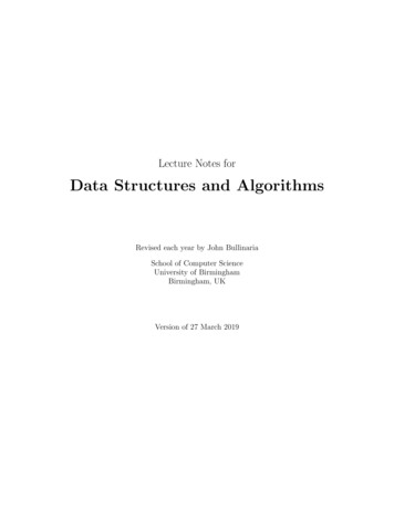
Chapter1Basic ConceptsThe term data structure is used to describe the way data is stored, and the termalgorithm is used to describe the way data is processed. Data structures andalgorithms are interrelated. Choosing a data structure affects the kind of algorithmyou might use, and choosing an algorithm affects the data structures we use.An Algorithm is a finite sequence of instructions, each of which has a clear meaningand can be performed with a finite amount of effort in a finite length of time. Nomatter what the input values may be, an algorithm terminates after executing afinite number of instructions.1.1.Introduction to Data Structures:Data structure is a representation of logical relationship existing between individual elements ofdata. In other words, a data structure defines a way of organizing all data items that considersnot only the elements stored but also their relationship to each other. The term data structureis used to describe the way data is stored.To develop a program of an algorithm we should select an appropriate data structure for thatalgorithm. Therefore, data structure is represented as:Algorithm Data structure ProgramA data structure is said to be linear if its elements form a sequence or a linear list. The lineardata structures like an array, stacks, queues and linked lists organize data in linear order. Adata structure is said to be non linear if its elements form a hierarchical classification where,data items appear at various levels.Trees and Graphs are widely used non-linear data structures. Tree and graph structuresrepresents hierarchial relationship between individual data elements. Graphs are nothing buttrees with certain restrictions removed.Data structures are divided into two types: Primitive data structures.Non-primitive data structures.Primitive Data Structures are the basic data structures that directly operate upon themachine instructions. They have different representations on different computers. Integers,floating point numbers, character constants, string constants and pointers come under thiscategory.Non-primitive data structures are more complicated data structures and are derived fromprimitive data structures. They emphasize on grouping same or different data items withrelationship between each data item. Arrays, lists and files come under this category. Figure1.1 shows the classification of data structures.Lecture Notes1Dept. of Information Technology
Da t a St r uc t ur e sNo n- Pr i mi t iv e Da t a St r uc t ur e sPr i mi t iv e Da t a St r uc t ur e sI nt e g erF l o atC h arP o i nt er sArr ay sL i st sL i n e ar L i st sSt ac k sFile sNo n- L i n e ar L i st sQueuesGr a p h sT re e sF i g ur e 1. 1. C l a s s if ic at i o n of Da t a St r uc t ur e s1.2.Data structures: Organization of dataThe collection of data you work with in a program have some kind of structure or organization.No matte how complex your data structures are they can be broken down into two fundamentaltypes: Contiguous Non-Contiguous.In contiguous structures, terms of data are kept together in memory (either RAM or in a file).An array is an example of a contiguous structure. Since each element in the array is locatednext to one or two other elements. In contrast, items in a non-contiguous structure andscattered in memory, but we linked to each other in some way. A linked list is an example of anon-contiguous data structure. Here, the nodes of the list are linked together using pointersstored in each node. Figure 1.2 below illustrates the difference between contiguous and noncontiguous structures.1231(a) Contiguous23(b) non-contiguousFigure 1.2 Contiguous and Non-contiguous structures comparedContiguous structures:Contiguous structures can be broken drawn further into two kinds: those that contain dataitems of all the same size, and those where the size may differ. Figure 1.2 shows example ofeach kind. The first kind is called the array. Figure 1.3(a) shows an example of an array ofnumbers. In an array, each element is of the same type, and thus has the same size.The second kind of contiguous structure is called structure, figure 1.3(b) shows a simplestructure consisting of a person’s name and age. In a struct, elements may be of different datatypes and thus may have different sizes.Lecture Notes2Dept. of Information Technology
For example, a person’s age can be represented with a simple integer that occupies two bytesof memory. But his or her name, represented as a string of characters, may require manybytes and may even be of varying length.Couples with the atomic types (that is, the single data-item built-in types such as integer, floatand pointers), arrays and structs provide all the “mortar” you need to built more exotic form ofdata structure, including the non-contiguous forms.int arr[3] {1, 2, 3};12struct cust data{int age;char name[20];};3cust data bill {21, “bill the student”};(a) Array21(b) struct“bill the student”Figure 1.3 Examples of contiguous structures.Non-contiguous structures:Non-contiguous structures are implemented as a collection of data-items, called nodes, whereeach node can point to one or more other nodes in the collection. The simplest kind of noncontiguous structure is linked list.A linked list represents a linear, one-dimension type of non-contiguous structure, where thereis only the notation of backwards and forwards. A tree such as shown in figure 1.4(b) is anexample of a two-dimensional non-contiguous structure. Here, there is the notion of up anddown and left and right.In a tree each node has only one link that leads into the node and links can only go down thetree. The most general type of non-contiguous structure, called a graph has no suchrestrictions. Figure 1.4(c) is an example of a graph.ABCAB(a) Linked ListCDAEBGCF(b) TreeDEF(c) graphGFigure 1.4. Examples of non-contiguous structuresLecture Notes3Dept. of Information Technology
Hybrid structures:If two basic types of structures are mixed then it is a hybrid form. Then one part contiguousand another part non-contiguous. For example, figure 1.5 shows how to implement a double–linked list using three parallel arrays, possibly stored a past from each other in memory.AList HeadBC(a) Conceptual StructureDPN1A342B403C014D12(b) Hybrid ImplementationFigure 1.5. A double linked list via a hybrid data structureThe array D contains the data for the list, whereas the array P and N hold the previous andnext “pointers’’. The pointers are actually nothing more than indexes into the D array. Forinstance, D[i] holds the data for node i and p[i] holds the index to the node previous to i,where may or may not reside at position i–1. Like wise, N[i] holds the index to the next node inthe list.1.3.Abstract Data Type (ADT):The design of a data structure involves more than just its organization. You also need to planfor the way the data will be accessed and processed – that is, how the data will be interpretedactually, non-contiguous structures – including lists, tree and graphs – can be implementedeither contiguously or non- contiguously like wise, the structures that are normally treated ascontiguously - arrays and structures – can also be implemented non-contiguously.The notion of a data structure in the abstract needs to be treated differently from what ever isused to implement the structure. The abstract notion of a data structure is defined in terms ofthe operations we plan to perform on the data.Considering both the organization of data and the expected operations on the data, leads to thenotion of an abstract data type. An abstract data type in a theoretical construct that consists ofdata as well as the operations to be performed on the data while hiding implementation.For example, a stack is a typical abstract data type. Items stored in a stack can only be addedand removed in certain order – the last item added is the first item removed. We call theseoperations, pushing and popping. In this definition, we haven’t specified have items are storedon the stack, or how the items are pushed and popped. We have only specified the validoperations that can be performed.For example, if we want to read a file, we wrote the code to read the physical file device. Thatis, we may have to write the same code over and over again. So we created what is knownLecture Notes4Dept. of Information Technology
today as an ADT. We wrote the code to read a file and placed it in a library for a programmer touse.As another example, the code to read from a keyboard is an ADT. It has a data structure,character and set of operations that can be used to read that data structure.To be made useful, an abstract data type (such as stack) has to be implemented and this iswhere data structure comes into ply. For instance, we might choose the simple data structureof an array to represent the stack, and then define the appropriate indexing operations toperform pushing and popping.1.4.Selecting a data structure to match the operation:The most important process in designing a problem involves choosing which data structure touse. The choice depends greatly on the type of operations you wish to perform.Suppose we have an application that uses a sequence of objects, where one of the mainoperations is delete an object from the middle of the sequence. The code for this is as follows:void delete (int *seg, int &n, int posn)// delete the item at position from an array of n elements.{if (n){int i posn;n--;while (i n){seq[i] seg[i 1];i ;}}return;}This function shifts towards the front all elements that follow the element at position posn. Thisshifting involves data movement that, for integer elements, which is too costly. However,suppose the array stores larger objects, and lots of them. In this case, the overhead for movingdata becomes high. The problem is that, in a contiguous structure, such as an array the logicalordering (the ordering that we wish to interpret our elements to have) is the same as thephysical ordering (the ordering that the elements actually have in memory).If we choose non-contiguous representation, however we can separate the logical ordering fromthe physical ordering and thus change one without affecting the other. For example, if we storeour collection of elements using a double–linked list (with previous and next pointers), we cando the deletion without moving the elements, instead, we just modify the pointers in eachnode. The code using double linked list is as follows:void delete (node * beg, int posn)//delete the item at posn from a list of elements.{int i posn;node *q beg;while (i && q){Lecture Notes5Dept. of Information Technology
i--;q q Æ next;}if (q){/* not at end of list, so detach P by making previous andnext nodes point to each other */node *p q - prev;node *n q - next;if (p)p - next n;if (n)n - prev P;}return;}The process of detecting a node from a list is independent of the type of data stored in thenode, and can be accomplished with some pointer manipulation as illustrated in figure below:AX200100Initial ListAC300XAFigure 1.6 Detaching a node from a listSince very little data is moved during this process, the deletion using linked lists will often befaster than when arrays are used.It may seem that linked lists are superior to arrays. But is that always true? There are tradeoffs. Our linked lists yield faster deletions, but they take up more space because they requiretwo extra pointers per element.1.5.AlgorithmAn algorithm is a finite sequence of instructions, each of which has a clear meaning and can beperformed with a finite amount of effort in a finite length of time. No matter what the inputvalues may be, an algorithm terminates after executing a finite number of instructions. Inaddition every algorithm must satisfy the following criteria:Input: there are zero or more quantities, which are externally supplied;Output: at least one quantity is produced;Lecture Notes6Dept. of Information Technology
Definiteness: each instruction must be clear and unambiguous;Finiteness: if we trace out the instructions of an algorithm, then for all cases the algorithm willterminate after a finite number of steps;Effectiveness: every instruction must be sufficiently basic that it can in principle be carried outby a person using only pencil and paper. It is not enough that each operation be definite, but itmust also be feasible.In formal computer science, one distinguishes between an algorithm, and a program. Aprogram does not necessarily satisfy the fourth condition. One important example of such aprogram for a computer is its operating system, which never terminates (except for systemcrashes) but continues in a wait loop until more jobs are entered.We represent an algorithm using pseudo language that is a combination of the constructs of aprogramming language together with informal English statements.1.6.Practical Algorithm design issues:Choosing an efficient algorithm or data structure is just one part of the design process. Next,will look at some design issues that are broader in scope. There are three basic design goalsthat we should strive for in a program:1.2.3.Try to save time (Time complexity).Try to save space (Space complexity).Try to have face.A program that runs faster is a better program, so saving time is an obvious goal. Like wise, aprogram that saves space over a competing program is considered desirable. We want to “saveface” by preventing the program from locking up or generating reams of garbled data.1.7.Performance of a program:The performance of a program is the amount of computer memory and time needed to run aprogram. We use two approaches to determine the performance of a program. One isanalytical, and the other experimental. In performance analysis we use analytical methods,while in performance measurement we conduct experiments.Time Complexity:The time needed by an algorithm expressed as a function of the size of a problem is called theTIME COMPLEXITY of the algorithm. The time complexity of a program is the amount ofcomputer time it needs to run to completion.The limiting behavior of the complexity as size increases is called the asymptotic timecomplexity. It is the asymptotic complexity of an algorithm, which ultimately determines thesize of problems that can be solved by the algorithm.Space Complexity:The space complexity of a program is the amount of memory it needs to run to completion. Thespace need by a program has the following components:Lecture Notes7Dept. of Information Technology
Instruction space: Instruction space is the space needed to store the compiled version of theprogram instructions.Data space: Data space is the space needed to store all constant and variable values. Dataspace has two components: Space needed by constants and simple variables in program.Space needed by dynamically allocated objects such as arrays and class instances.Environment stack space: The environment stack is used to save information needed toresume execution of partially completed functions.Instruction Space: The amount of instructions space that is needed depends on factors suchas: The compiler used to complete the program into machine code. The compiler options in effect at the time of compilation The target computer.1.8.Classification of AlgorithmsIf ‘n’ is the number of data items to be processed or degree of polynomial or the size of the fileto be sorted or searched or the number of nodes in a graph etc.1Next instructions of most programs are executed once or at most only a few times.If all the instructions of a program have this property, we say that its running timeis a constant.Log nWhen the running time of a program is logarithmic, the program gets slightlyslower as n grows. This running time commonly occurs in programs that solve a bigproblem by transforming it into a smaller problem, cutting the size by someconstant fraction., When n is a million, log n is a doubled whenever n doubles, logn increases by a constant, but log n does not double until n increases to n2.nWhen the running time of a program is linear, it is generally the case that a smallamount of processing is done on each input element. This is the optimal situationfor an algorithm that must process n inputs.n. log nThis running time arises for algorithms but solve a problem by breaking it up intosmaller sub-problems, solving them independently, and then combining thesolutions. When n doubles, the running time more than doubles.n2When the running time of an algorithm is quadratic, it is practical for use only onrelatively small problems. Quadratic running times typically arise in algorithms thatprocess all pairs of data items (perhaps in a double nested loop) whenever ndoubles, the running time increases four fold.n3Similarly, an algorithm that process triples of data items (perhaps in a triple–nested loop) has a cubic running time and is practical for use only on smallproblems. Whenever n doubles, the running time increases eight fold.2nFew algorithms with exponential running time are likely to be appropriate forpractical use, such algorithms arise naturally as “brute–force” solutions toproblems. Whenever n doubles, the running time squares.Lecture Notes8Dept. of Information Technology
1.9.Complexity of AlgorithmsThe complexity of an algorithm M is the function f(n) which gives the running time and/orstorage space requirement of the algorithm in terms of the size ‘n’ of the input data. Mostly,the storage space required by an algorithm is simply a multiple of the data size ‘n’. Complexityshall refer to the running time of the algorithm.The function f(n), gives the running time of an algorithm, depends not only on the size ‘n’ ofthe input data but also on the particular data. The complexity function f(n) for certain casesare:1.Best Case:The minimum possible value of f(n) is called the best case.2.Average Case:The expected value of f(n).3.Worst Case:The maximum value of f(n) for any key possible input.The field of computer science, which studies efficiency of algorithms, is known as analysis ofalgorithms.Algorithms can be evaluated by a variety of criteria. Most often we shall be interested in therate of growth of the time or space required to solve larger and larger instances of a problem.We will associate with the problem an integer, called the size of the problem, which is ameasure of the quantity of input data.1.10. Rate of GrowthBig–Oh (O), Big–Omega (Ω), Big–Theta (Θ) and Little–Oh1.T(n) O(f(n)), (pronounced order of or big oh), says that the growth rate of T(n) isless than or equal ( ) that of f(n)2.T(n) Ω(g(n)) (pronounced omega), says that the growth rate of T(n) is greater thanor equal to ( ) that of g(n)3.T(n) Θ(h(n)) (pronounced theta), says that the growth rate of T(n) equals ( ) thegrowth rate of h(n) [if T(n) O(h(n)) and T(n) Ω (h(n)]4.T(n) o(p(n)) (pronounced little oh), says that the growth rate of T(n) is less than thegrowth rate of p(n) [if T(n) O(p(n)) and T(n) Θ (p(n))].Some Examples:2n22n22n22n2 5n5n5n5n––––6666 O(2n)O(n3)O(n2)O(n)2n22n22n22n2 5n5n5n5n––––6666 Θ(2n)Θ(n3)Θ(n2)Θ(n)2n22n22n22n2 5n5n5n5n––––6666 Ω(2n)Ω(n3)Ω(n2)Ω(n)2n22n22n22n2 5n5n5n5n––––6666 o(2n)o(n3)o(n2)o(n)Lecture Notes9Dept. of Information Technology
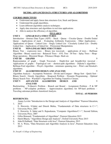
1.11. Analyzing AlgorithmsSuppose ‘M’ is an algorithm, and suppose ‘n’ is the size of the input data. Clearly thecomplexity f(n) of M increases as n increases. It is usually the rate of increase of f(n) we wantto examine. This is usually done by comparing f(n) with some standard functions. The mostcommon computing times are:O(1), O(log2 n), O(n), O(n. log2 n), O(n2), O(n3), O(2n), n! and nnNumerical Comparison of Different AlgorithmsThe execution time for six of the typical functions is given below:S.Nolog nnn. log 256409665536Graph of log n, n, n log n, n2, n3, 2n, n! and nnO(log n) does not depend on the base of the logarithm. To simplify the analysis, the conventionwill not have any particular units of time. Thus we throw away leading constants. We will alsothrow away low–order terms while computing a Big–Oh running time. Since Big-Oh is an upperbound, the answer provided is a guarantee that the program will terminate within a certaintime period. The program may stop earlier than this, but never later.Lecture Notes10Dept. of Information Technology
One way to compare the function f(n) with these standard function is to use the functional ‘O’notation, suppose f(n) and g(n) are functions defined on the positive integers with the propertythat f(n) is bounded by some multiple g(n) for almost all ‘n’. Then,f(n) O(g(n))Which is read as “f(n) is of order g(n)”. For example, the order of complexity for: Linear search is O(n)Binary search is O(log n)Bubble sort is O(n2)Quick sort is O(n log n)For example, if the first program takes 100n2 milliseconds. While the second taken 5n3milliseconds. Then might not 5n3 program better than 100n2 program?As the programs can be evaluated by comparing their running time functions, with constants byproportionality neglected. So, 5n3 program be better than the 100n2 program.5 n3/100 n2 n/20for inputs n 20, the program with running time 5n3 will be faster those the one with runningtime 100 n2.Therefore, if the program is to be run mainly on inputs of small size, we would indeed preferthe program whose running time was O(n3)However, as ‘n’ gets large, the ratio of the running times, which is n/20, gets arbitrarily larger.Thus, as the size of the input increases, the O(n3) program will take significantly more timethan the O(n2) program. So it is always better to prefer a program whose running time with thelower growth rate. The low growth rate function’s such as O(n) or O(n log n) are always better.Exercises1. Define algorithm.2. State the various steps in developing algorithms?3. State the properties of algorithms.4. Define efficiency of an algorithm?5. State the various methods to estimate the efficiency of an algorithm.6. Define time complexity of an algorithm?7. Define worst case of an algorithm.8. Define average case of an algorithm.9. Define best case of an algorithm.10. Mention the various spaces utilized by a program.Lecture Notes11Dept. of Information Technology
11. Define space complexity of an algorithm.12. State the different memory spaces occupied by an algorithm.Multiple Choice Questions1.is a step-by-step recipe for solving an instance of problem.A. AlgorithmB. ComplexityC. PseudocodeD. Analysis[A]2.is used to describe the algorithm, in less formal language.A. Cannot be definedB. Natural LanguageC. PseudocodeD. None[C]3.of an algorithm is the amount of time (or the number of steps)needed by a program to complete its task.A. Space ComplexityB. Dynamic ProgrammingC. Divide and ConquerD. Time Complexity[D]4.of a program is the amount of memory used at once by thealgorithm until it completes its execution.[C][A]A. Divide and ConquerC. Space Complexity5.B. Time ComplexityD. Dynamic Programmingis used to define the worst-case running time of an algorithm.A. Big-Oh notationB. Cannot be definedC. ComplexityD. AnalysisLecture Notes12Dept. of Information Technology
Chapter2RecursionRecursion is deceptively simple in statement but exceptionallycomplicated in implementation. Recursive procedures work fine in manyproblems. Many programmers prefer recursion through simpleralternatives are available. It is because recursion is elegant to usethrough it is costly in terms of time and space. But using it is one thingand getting involved with it is another.In this unit we will look at “recursion” as a programmer who not onlyloves it but also wants to understand it! With a bit of involvement it isgoing to be an interesting reading for you.2.1.Introduction to Recursion:A function is recursive if a statement in the body of the function calls itself. Recursion isthe process of defining something in terms of itself. For a computer language to berecursive, a function must be able to call itself.For example, let us consider the function factr() shown below, which computers thefactorial of an integer.#include stdio.h int factorial (int);main(){int num, fact;printf (“Enter a positive integer value: ");scanf (“%d”, &num);fact factorial (num);printf ("\n Factorial of %d %5d\n", num, fact);}int factorial (int n){int result;if (n 0)return (1);elseresult n * factorial (n-1);}return (result);A non-recursive or iterative version for finding the factorial is as follows:factorial (int n){int i, result 1;if (n 0)Lecture Notes13Dept. of Information Technology
return (result);else{for (i 1; i n; i )result result * i;}return (result);}The operation of the non-recursive version is clear as it uses a loop starting at 1 andending at the target value and progressively multiplies each number by the movingproduct.When a function calls itself, new local variables and parameters are allocated storageon the stack and the function code is executed with these new variables from the start.A recursive call does not make a new copy of the function. Only the arguments andvariables are new. As each recursive call retu
Figure 1.2 C ontiguous and Non-contiguous structures compared Contiguous structures: Contiguous structures can be broken drawn further into two kinds: those that contain data items of all the same size, and those where the size may differ. Figure 1.2 shows example of each kind. The first kind is called the array.