Transcription
Introduction to Complex AnalysisMichael Taylor1
2ContentsChapter 1. Basic calculus in the complex domain0.1.2.3.4.I.Complex numbers, power series, and exponentialsHolomorphic functions, derivatives, and path integralsHolomorphic functions defined by power seriesExponential and trigonometric functions: Euler’s formulaSquare roots, logs, and other inverse functionsπ 2 is irrationalChapter 2. Going deeper – the Cauchy integral theorem and consequences5. The Cauchy integral theorem and the Cauchy integral formula6. The maximum principle, Liouville’s theorem, and the fundamental theorem of algebra7. Harmonic functions on planar regions8. Morera’s theorem, the Schwarz reflection principle, and Goursat’s theorem9. Infinite products10. Uniqueness and analytic continuation11. Singularities12. Laurent seriesC. Green’s theoremF. The fundamental theorem of algebra (elementary proof)L. Absolutely convergent seriesChapter 3. Fourier analysis and complex function theory13.14.15.H.N.G.Fourier series and the Poisson integralFourier transformsLaplace transforms and Mellin transformsInner product spacesThe matrix exponentialThe Weierstrass and Runge approximation theoremsChapter 4. Residue calculus, the argument principle, and two very specialfunctions16.17.18.19.J.S.Residue calculusThe argument principleThe Gamma functionThe Riemann zeta function and the prime number theoremEuler’s constantHadamard’s factorization theorem
3Chapter 5. Conformal maps and geometrical aspects of complex function theory20.21.22.23.24.25.26.27.28.29.D.E.Conformal mapsNormal familiesThe Riemann sphere (and other Riemann surfaces)The Riemann mapping theoremBoundary behavior of conformal mapsCovering mapsThe disk covers C \ {0, 1}Montel’s theoremPicard’s theoremsHarmonic functions IISurfaces and metric tensorsPoincaré metricsChapter 6. Elliptic functions and elliptic integrals30.31.32.33.34.K.Periodic and doubly periodic functions - infinite series representationsThe Weierstrass in elliptic function theoryTheta functions and Elliptic integrals The Riemann surface of q(ζ)Rapid evaluation of the Weierstrass -functionChapter 7. Complex analysis and differential equations35. Bessel functions36. Differential equations on a complex domainO. From wave equations to Bessel and Legendre equationsAppendicesA.B.P.M.R.Q.Metric spaces, convergence, and compactnessDerivatives and diffeomorphismsThe Laplace asymptotic method and Stirling’s formulaThe Stieltjes integralAbelian theorems and Tauberian theoremsCubics, quartics, and quintics
4PrefaceThis text is designed for a first course in complex analysis, for beginning graduate students, or well prepared undergraduates, whose background includes multivariable calculus,linear algebra, and advanced calculus. In this course the student will learn that all the basicfunctions that arise in calculus, first derived as functions of a real variable, such as powersand fractional powers, exponentials and logs, trigonometric functions and their inverses,and also many new functions that the student will meet, are naturally defined for complexarguments. Furthermore, this expanded setting reveals a much richer understanding ofsuch functions.Care is taken to introduce these basic functions first in real settings. In the openingsection on complex power series and exponentials, in Chapter 1, the exponential functionis first introduced for real values of its argument, as the solution to a differential equation.This is used to derive its power series, and from there extend it to complex argument.Similarly sin t and cos t are first given geometrical definitions, for real angles, and theEuler identity is established based on the geometrical fact that eit is a unit-speed curve onthe unit circle, for real t. Then one sees how to define sin z and cos z for complex z.The central objects in complex analysis are functions that are complex-differentiable(i.e., holomorphic). One goal in the early part of the text is to establish an equivalencebetween being holomorphic and having a convergent power series expansion. Half of thisequivalence, namely the holomorphy of convergent power series, is established in Chapter1.Chapter 2 starts with two major theoretical results, the Cauchy integral theorem, andits corollary, the Cauchy integral formula. These theorems have a major impact on theentire rest of the text, including the demonstration that if a function f (z) is holomorphicon a disk, then it is given by a convergent power series on that disk. A useful variant ofsuch power series is the Laurent series, for a function holomorphic on an annulus.The text segues from Laurent series to Fourier series, in Chapter 3, and from there to theFourier transform and the Laplace transform. These three topics have many applications inanalysis, such as constructing harmonic functions, and providing other tools for differentialequations. The Laplace transform of a function has the important property of beingholomorphic on a half space. It is convenient to have a treatment of the Laplace transformafter the Fourier transform, since the Fourier inversion formula serves to motivate andprovide a proof of the Laplace inversion formula.Results on these transforms illuminate the material in Chapter 4. For example, thesetransforms are a major source of important definite integrals that one cannot evaluate byelementary means, but that are amenable to analysis by residue calculus, a key applicationof the Cauchy integral theorem. Chapter 4 starts with this, and proceeds to the study oftwo important special functions, the Gamma function and the Riemann zeta function.The Gamma function, which is the first “higher” transcendental function, is essentiallya Laplace transform. The Riemann zeta function is a basic object of analytic number
5theory, arising in the study of prime numbers. One sees in Chapter 4 roles of Fourieranalysis, residue calculus, and the Gamma function in the study of the zeta function. Forexample, a relation between Fourier series and the Fourier transform, known as the Poissonsummation formula, plays an important role in its study.In Chapter 5, the text takes a geometrical turn, viewing holomorphic functions asconformal maps. This notion is pursued not only for maps between planar domains,but also for maps to surfaces in R3 . The standard case is the unit sphere S 2 , and theassociated stereographic projection. The text also considers other surfaces. It constructsconformal maps from planar domains to general surfaces of revolution, deriving for the mapa first-order differential equation, nonlinear but separable. These surfaces are discussedb C { } is also discussed asas examples of Riemann surfaces. The Riemann sphere C2a Riemann surface, conformally equivalent to S . One sees the group of linear fractionalb and certain subgroups astransformations as a group of conformal automorphisms of C,groups of conformal automorphisms of the unit disk and of the upper half plane.We also bring in the notion of normal families, to prove the Riemann mapping theorem.Application of this theorem to a special domain, together with a reflection argument, showsthat there is a holomorphic covering of C \ {0, 1} by the unit disk. This leads to key resultsof Picard and Montel, and applications to the behavior of iterations of holomorphic mapsb C,b and the Julia sets that arise.R:CThe treatment of Riemann surfaces includes some differential geometric material. Inan appendix to Chapter 5, we introduce the concept of a metric tensor, and show how itis associated to a surface in Euclidean space, and how the metric tensor behaves undersmooth mappings, and in particular how this behavior characterizes conformal mappings.We discuss the notion of metric tensors beyond the setting of metrics induced on surfacesin Euclidean space. In particular, we introduce a special metric on the unit disk, calledthe Poincaré metric, which has the property of being invariant under all conformal automorphisms of the disk. We show how the geometry of the Poincaré metric leads to anotherproof of Picard’s theorem, and also provides a different perspective on the proof of theRiemann mapping theorem.The text next examines elliptic functions, in Chapter 6. These are doubly periodicfunctions on C, holomorphic except at poles (that is, meromorphic). Such a functioncan be regarded as a meromorphic function on the torus TΛ C/Λ, where Λ C is alattice. A prime example is the Weierstrass function Λ (z), defined by a double series.Analysis shows that ′Λ (z)2 is a cubic polynomial in Λ (z), so the Weierstrass functioninverts an elliptic integral. Elliptic integrals arise in many situations in geometry andmechanics, including arclengths of ellipses and pendulum problems, to mention two basiccases. The analysis of general elliptic integrals leads to the problem of finding the latticewhose associated elliptic functions are related to these integrals. This is the Abel inversionproblem. Section 34 of the text tackles this problem by constructing the Riemann surfaceassociated to p(z), where p(z) is a cubic or quartic polynomial.Early in this text, the exponential function was defined by a differential equation andgiven a power series solution, and these two characterizations were used to develop itsproperties. Coming full circle, we devote Chapter 7 to other classes of differential equations
6and their solutions. We first study a special class of functions known as Bessel functions,characterized as solutions to Bessel equations. Part of the central importance of thesefunctions arises from their role in producing solutions to partial differential equations inseveral variables, as explained in an appendix. The Bessel functions for real values oftheir arguments arise as solutions to wave equations, and for imaginary values of theirarguments they arise as solutions to diffusion equations. Thus it is very useful that theycan be understood as holomorphic functions of a complex variable. Next, Chapter 7 dealswith more general differential equations on a complex domain. Results include constructingsolutions as convergent power series and the analytic continuation of such solutions to largerdomains. General results here are used to put the Bessel equations in a larger context. Thisincludes a study of equations with “regular singular points.” Other classes of equationswith regular singular points are presented, particularly hypergeometric equations.The text ends with a short collection of appendices. Some of these survey backgroundmaterial that the reader might have seen in an advanced calculus course, including materialon convergence and compactness, and differential calculus of several variables. Othersdevelop tools that prove useful in the text, the Laplace asymptotic method, the Stieltjesintegral, and results on Abelian and Tauberian theorems. The last appendix shows how tosolve cubic and quartic equations via radicals, and introduces a special function, called theBring radical, to treat quintic equations. (In §36 the Bring radical is shown to be given interms of a generalized hypergeometric function.)As indicated in the discussion above, while the first goal of this text is to present thebeautiful theory of functions of a complex variable, we have the further objective of placingthis study within a broader mathematical framework. Examples of how this text differsfrom many others in the area include the following.1) A greater emphasis on Fourier analysis, both as an application of basic results in complexanalysis and as a tool of more general applicability in analysis. We see the use of Fourierseries in the study of harmonic functions. We see the influence of the Fourier transformon the study of the Laplace transform, and then the Laplace transform as a tool in thestudy of differential equations.2) The use of geometrical techniques in complex analysis. This clarifies the study of conformal maps, extends the usual study to more general surfaces, and shows how geometricalconcepts are effective in classical problems, from the Riemann mapping theorem to Picard’stheorem. An appendix discusses applications of the Poincaré metric on the disk.3) Connections with differential equations. The use of techniques of complex analysis tostudy differential equations is a strong point of this text. This important area is frequentlyneglected in complex analysis texts, and the treatments one sees in many differential equations texts are often confined to solutions for real variables, and may furthermore lack acomplete analysis of crucial convergence issues. Material here also provides a more detailedstudy than one usually sees of significant examples, such as Bessel functions.
74) Special functions. In addition to material on the gamma function and the Riemann zetafunction, the text has a detailed study of elliptic functions and Bessel functions, and alsomaterial on Airy functions, Legendre functions, and hypergeometric functions.We follow this introduction with a record of some standard notation that will be usedthroughout this text.AcknowledgmentThanks to Shrawan Kumar for testing this text in his Complex Analysis course, for pointingout corrections, and for other valuable advice.
8Some Basic NotationR is the set of real numbers.C is the set of complex numbers.Z is the set of integers.Z is the set of integers 0.N is the set of integers 1 (the “natural numbers”).x R means x is an element of R, i.e., x is a real number.(a, b) denotes the set of x R such that a x b.[a, b] denotes the set of x R such that a x b.{x R : a x b} denotes the set of x in R such that a x b.[a, b) {x R : a x b} and (a, b] {x R : a x b}.z x iy if z x iy C, x, y R.Ω denotes the closure of the set Ω.f : A B denotes that the function f takes points in the set A to pointsin B. One also says f maps A to B.x x0 means the variable x tends to the limit x0 .f (x) O(x) means f (x)/x is bounded. Similarly g(ε) O(εk ) meansg(ε)/εk is bounded.f (x) o(x) as x 0 (resp., x ) means f (x)/x 0 as x tends to thespecified limit.S sup an means S is the smallest real number that satisfies S an for all n.nIf there is no such real number then we take S .()lim sup ak lim sup ak .k n k n
9Chapter 1. Basic calculus in the complex domainThis first chapter introduces the complex numbers and begins to develop results on thebasic elementary functions of calculus, first defined for real arguments, and then extendedto functions of a complex variable.An introductory §0 defines the algebraic operations on complex numbers, say z x iyand w u iv, discusses the magnitude z of z, defines convergence of infinite sequencesand series, and derives some basic facts about power series(1.0.1)f (z) ak z k ,k 0such as the fact that if this converges for z z0 , then it converges absolutely for z R z0 , to a continuous function. It is also shown that, for z t real,(1.0.2)f ′ (t) for R t R.kak tk 1 ,k 1Here we allow ak C. As an application, we consider the differential equation(1.0.3)dx x,dtx(0) 1,and deduce from (1.0.2) that a solution is given by x(t) define the exponential function(1.0.4) k 0tk /k!. Having this, we 1 kz ,e k!zk 0and use these observations to deduce that, whenever a C,(1.0.5)d ate aeat .dtWe use this differential equation to derive further properties of the exponential function.While §0 develops calculus for complex valued functions of a real variable, §1 introducescalculus for complex valued functions of a complex variable. We define the notion of complex differentiability. Given an open set Ω C, we say a function f : Ω C is holomorphicon Ω provided it is complex differentiable, with derivative f ′ (z), and f ′ is continuous on Ω.Writing f (z) u(z) iv(z), we discuss the Cauchy-Riemann equations for u and v. Wealso introduce the path integral and provide some versions of the fundamental theorem ofcalculus in the complex setting. (More definitive results will be given in Chapter 2.)
10Typically the functions we study are defined on a subset Ω C that is open. That is,if z0 Ω, there exists ε 0 such that z Ω whenever z z0 ε. Other terms we usefor a nonempty open set are “domain” and “region.” These terms are used synonymouslyin this text.In §2 we return to convergent power series and show they produce holomorphic functions.We extend results of §0 from functions of a real variable to functions of a complex variable.Section 3 returns to the exponential function ez , defined above. We extend (1.0.5) tod aze aeaz .dz(1.0.6)We show that t 7 et maps R one-to-one and onto (0, ), and define the logarithm on(0, ), as its inverse:(1.0.7)x et t log x.We also examine the behavior of γ(t) eit , for t R, showing that this is a unit-speedcurve tracing out the unit circle. From this we deduce Euler’s formula,(1.0.8)eit cos t i sin t.This leads to a direct, self-contained treatment of the trigonometric functions.In §4 we discuss inverses to holomorphic functions. In particular, we extend the logarithm from (0, ) to C \ ( , 0], as a holomorphic function. We define fractional powers(1.0.9)z a ea log z ,a C, z C \ ( , 0],and investigate their basic properties. We also discuss inverse trigonometric functions inthe complex plane.The number π arises in §3 as half the length of the unit circle, or equivalently thesmallest positive number satisfying(1.0.10)eπi 1.This is possibly the most intriguing number in mathematics. It will appear many timesover the course of this text. One of our goals will be to obtain accurate numerical approximations to π. In another vein, in Appendix I we show that π 2 is irrational.
110. Complex numbers, power series, and exponentialsA complex number has the form(0.1)z x iy,where x and y are real numbers. These numbers make up the complex plane, which isjust the xy-plane with the real line forming the horizontal axis and the real multiples of iforming the vertical axis. See Figure 0.1. We write(0.2)x Re z,y Im z.We write x, y R and z C. We identify x R with x i0 C. If also w u iv withu, v R, we have addition and multiplication, given byz w (x u) i(y v),(0.3)zw (xu yv) i(xv yu),the latter rule containing the identityi2 1.(0.4)One readily verifies the commutative laws(0.5)z w w z,zw wz,the associative laws (with also c C)(0.6)z (w c) (z w) c,z(wc) (zw)c,and the distributive law(0.7)c(z w) cz cw,as following from their counterparts for real numbers. If c ̸ 0, we can perform divisionby c,z w z wc.cSee (0.13) for a neat formula.For z x iy, we define z to be the distance of z from the origin 0, via the Pythagoreantheorem: (0.8) z x2 y 2 .
12Note that(0.9) z 2 z z,where z x iy,is called the complex conjugate of z. One readily checks that(0.10)z z 2 Re z,z z 2i Im z,and(0.11)z w z w,zw z w.Hence zw 2 zwz w z 2 w 2 , so zw z · w .(0.12)We also have, for c ̸ 0,z1 2 zc.c c (0.13)The following result is known as the triangle inequality, as Figure 0.2 suggests.Proposition 0.1. Given z, w C,(0.14) z w z w .Proof. We compare the squares of the two sides: z w 2 (z w)(z w)(0.15) zz ww zw wz z 2 w 2 2 Re(zw),while(0.16)( z w )2 z 2 w 2 2 z · w z 2 w 2 2 zw .Thus (0.14) follows from the inequality Re(zw) zw , which in turn is immediate fromthe definition (0.8). (For any ζ C, Re ζ ζ .)We can define convergence of a sequence (zn ) in C as follows. We say(0.17)zn z if and only if zn z 0,
13the latter notion involving convergence of a sequence of real numbers. Clearly if zn xn iyn and z x iy, with xn , yn , x, y R, then(0.18)zn z if and only if xn x and yn y.One readily verifies that(0.19)zn z, wn w zn wn z w and zn wn zw,as a consequence of their counterparts for sequences of real numbers.A related notion is that a sequence (zn ) in C is Cauchy if and only if(0.19A) zn zm 0 as m, n .As in (0.18), this holds if and only if (xn ) and (yn ) are Cauchy in R. The following is animportant fact.(0.19B)Each Cauchy sequence in C converges.This follows from the fact that(0.19C)each Cauchy sequence in R converges.A detailed presentation of the field R of real numbers, including a proof of (0.19C), is givenin Chapter 1 of [T0].We can define the notion of convergence of an infinite series(0.20) zkk 0as follows. For each n Z , set(0.21)sn n zk .k 0Then (0.20) converges if and only if the sequence (sn ) converges:(0.22)sn w zk w.k 0Note that sn m sn n m k n 1(0.23) n m k n 1Using this, we can establish the following.zk zk .
14Lemma 0.1A. Assume that (0.24) zk ,k 0i.e., there exists A such thatN (0.24A) zk A, N.k 0Then the sequence (sn ) given by (0.21) is Cauchy, hence the series (0.20) is convergent.Proof. If (sn ) is not Cauchy, there exist a 0, nν , and mν 0 such that snν mν snν a.Passing to a subsequence, one can assume that nν 1 nν mν . Then (0.23) impliesm ν nν zk νa, ν,k 0contradicting (0.24A).If (0.24) holds, we say the series (0.20) is absolutely convergent.An important class of infinite series is the class of power series (0.25)ak z k ,k 0with ak C. Note that if z1 ̸ 0 and (0.25) converges for z z1 , then there exists C such that ak z1k C,(0.25A) k.Hence, if z r z1 , r 1, we have(0.26) k 0 ak z Ck k 0rk C ,1 rthe last identity being the classical geometric series computation. See Exercise 3 below.This yields the following.
15Proposition 0.2. If (0.25) converges for some z1 ̸ 0, then either this series is absolutelyconvergent for all z C, or there is some R (0, ) such that the series is absolutelyconvergent for z R and divergent for z R.We call R the radius of convergence of (0.25). In case of convergence for all z, we saythe radius of convergence is infinite. If R 0 and (0.25) converges for z R, it definesa function(0.27)f (z) ak z k ,z DR ,k 0on the disk of radius R centered at the origin,DR {z C : z R}.(0.28)Proposition 0.3. If the series (0.27) converges in DR , then f is continuous on DR , i.e.,given zn , z DR ,zn z f (zn ) f (z).(0.29)Proof. For each z DR , there exists S R such that z DS , so it suffices to show thatf is continuous on DS whenever 0 S R. Pick T such that S T R. We know thatthere exists C such that ak T k C for all k. Hencez DS ak z k C(0.30)( S )kT.For each N , writef (z) SN (z) RN (z),(0.31)SN (z) N ak z k ,RN (z) k 0 ak z k .k N 1Each SN (z) is a polynomial in z, and it follows readily from (0.19) that SN is continuous.Meanwhile,(0.32)z DS RN (z) k N 1 ( )k S ak z C CεN ,Tkk N 1and εN 0 as N , independently of z DS . Continuity of f on DS follows, as aconsequence of the next lemma.
16Lemma 0.3A. Let SN : DS C be continuous functions. Assume f : DS C andSN f uniformly on DS , i.e., SN (z) f (z) δN , z DS ,(0.32A)δN 0, as N .Then f is continuous on DS .Proof. Let zn z in DS . We need to show that, given ε 0, there exists M M (ε) such that f (z) f (zn ) ε, n M.To get this, pick N such that (0.32A) holds with δN ε/3. Now use continuity of SN , todeduce that there exists M such that SN (z) SN (zn ) ε,3 n M.It follows that, for n M , f (z) f (zn ) f (z) SN (z) SN (z) SN (zn ) SN (zn ) f (zn ) ε ε ε ,3 3 3as desired.Remark. The estimate (0.32) says the series (0.27) converges uniformly on DS , for eachS R.A major consequence of material developed in §§1–5 will be that a function on DRis given by a convergent power series (0.27) if and only if f has the property of beingholomorphic on DR (a property that is defined in §1). We will be doing differential andintegral calculus on such functions. In this preliminary section, we restrict z to be real,and do some calculus, starting with the following.Proposition 0.4. Assume ak C and(0.33)f (t) a k tkk 0converges for real t satisfying t R. Then f is differentiable on the interval R t R,and(0.34)′f (t) kak tk 1 ,k 1the latter series being absolutely convergent for t R.
17We first check absolute convergence of the series (0.34). Let S T R. Convergenceof (0.33) implies there exists C such that ak T k C,(0.35) k.Hence, if t S, kak tk 1 (0.35A)C ( S )kk.STThe absolute convergence of (0.36)for r 1,krk ,k 0follows from the ratio test. (See Exercises 4–5 below.) Hence(0.37)g(t) kak tk 1k 1is continuous on ( R, R). To show that f ′ (t) g(t), by the fundamental theorem ofcalculus, it is equivalent to show tg(s) ds f (t) f (0).(0.38)0The following result implies this.Proposition 0.5. Assume bk C and(0.39)g(t) bk tkk 0converges for real t, satisfying t R. Then, for t R, (0.40)tg(s) ds 0 bk k 1t,k 1k 0the series being absolutely convergent for t R.Proof. Since, for t R,(0.41)bk k 1 R bk tk ,tk 1
18convergence of the series in (0.40) is clear. Next, parallel to (0.31), writeg(t) SN (t) RN (t),(0.42)SN (t) N kbk t ,RN (t) k 0 bk tk .k N 1Parallel to (0.32), if we pick S R, we have(0.43) t S RN (t) CεN 0 as N ,so tN bk k 1t RN (s) ds,g(s) ds k 10t(0.44)0k 0and tRN (s) ds (0.45)0t RN (s) ds CRεN ,0for t S. This gives (0.40).We use Proposition 0.4 to solve some basic differential equations, starting with(0.46)f ′ (t) f (t),f (0) 1.We look for a solution as a power series, of the form (0.33). If there is a solution of thisform, (0.34) requires(0.47)a0 1,ak 1 ak,k 1i.e., ak 1/k!, where k! k(k 1) · · · 2 · 1. We deduce that (0.46) is solved by(0.48)f (t) et 1 kt ,k!t R.k 0This defines the exponential function et . Convergence for all t follows from the ratio test.(Cf. Exercise 4 below.) More generally, we define(0.49) 1 ke z ,k!zk 0z C.
19Again the ratio test shows that this series is absolutely convergent for all z C. Anotherapplication of Proposition 0.4 shows that(0.50)eat akk 0k!tksolvesd ate aeat ,dt(0.51)whenever a C.We claim that eat is the only solution tof ′ (t) af (t),(0.52)f (0) 1.To see this, compute the derivative of e at f (t):)d ( ate f (t) ae at f (t) e at af (t) 0,dt(0.53)where we use the product rule, (0.51) (with a replaced by a), and (0.52). Thus e at f (t)is independent of t. Evaluating at t 0 givese at f (t) 1,(0.54) t R,whenever f (t) solves (0.52). Since eat solves (0.52), we have e at eat 1, hencee at (0.55)1,eat t R, a C.Thus multiplying both sides of (0.54) by eat gives the asserted uniqueness:f (t) eat ,(0.56) t R.We can draw further useful conclusions by applying d/dt to products of exponentials.Let a, b C. Then(0.57)d ( at bt (a b)t )e e edt ae at e bt e(a b)t be at e bt e(a b)t (a b)e at e bt e(a b)t 0,so again we are differentiating a function that is independent of t. Evaluation at t 0gives(0.58)e at e bt e(a b)t 1, t R.
20Using (0.55), we gete(a b)t eat ebt ,(0.59) t R, a, b C,or, setting t 1, a, b C.ea b ea eb ,(0.60)We will resume study of the exponential function in §3, and derive further importantproperties.Exercises1. Supplement (0.19) with the following result. Assume there exists A 0 such that zn A for all n. Thenzn z (0.61)11 .znz2. Show that z 1 z k 0, as k .(0.62)Hint. Deduce (0.62) from the assertion0 s 1 ksk is bounded, for k N.(0.63)Note that this is equivalent to(0.64)a 0 kis bounded, for k N.(1 a)kShow that(0.65)(1 a)k (1 a) · · · (1 a) 1 ka, a 0, k N.Use this to prove (0.64), hence (0.63), hence (0.62).3. Letting sn (0.66) nk 0rk , write the series for rsn and show that(1 r)sn 1 rn 1,1 rn 1hence sn .1 r
21Deduce that(0.67)1, as n ,1 r0 r 1 sn as stated in (0.26). More generally, show that(0.67A) k 0zk 1,1 zfor z 1.4. This exercise discusses the ratio test, mentioned in connection with the infinite series(0.36) and (0.49). Consider the infinite series (0.68)ak ,ak C.k 0Assume there exists r 1 and N such thatk N (0.69)ak 1 r.akShow that (0.70) ak .k 0Hint. Show that(0.71) ak aN k N rℓ ℓ 0 aN .1 r5. In case(0.72)ak zk,k!show that for each z C, there exists N such that (0.69) holds, with r 1/2. Alsoshow that the ratio test applies to(0.73)ak kz k , z 1.6. This exercise discusses the integral test for absolute convergence of an infinite series,
22which goes as follows. Let f be a positive, monotonically decreasing, continuous functionon [0, ), and suppose ak f (k). Then ak f (t) dt .0k 0Prove this.Hint. Use N N ak f (t) dt 0k 1N 1 ak .k 07. Use the integral test to show that, if a 0, 1 a 1.ann 18. This exercise deals with alternating series. Assume bk 0. Show that ( 1)k bk is convergent,k 0be showing that, for m, n 0,n m ( 1)k bk bn .k n9. Show that k 1 ( 1)k/k is convergent, but not absolutely convergent.10. Show that if f, g : (a, b) C are differentiable, then)d(f (t)g(t) f ′ (t)g(t) f (t)g ′ (t).dt(0.74)Note the use of this identity in (0.53) and (0.57).11. Use the results of Exercise 10 to show, by induction on k, thatd kt ktk 1 ,dt(0.75)k 1, 2, 3, . . . ,hence tsk ds (0.76)01 k 1t,k 1k 0, 1, 2, . . . .
23Note the use of these identities in (0.44), leading to many of the identities in (0.34)–(0.51).12. Considerφ(z) z 1.z 1Show thatφ : C \ { 1} C \ {1}is continuous, one-to-one, and onto. Show that, if Ω {z C : Re z 0} and D {z C : z 1}, thenφ : Ω D and φ : Ω D \ {1}are one-to-one and onto.Remark. This exercise is relevant to material in Exercise 7 of §4. The result here is aspecial case of important results on linear fractional transformations, discussed at leng
12. Laurent series C. Green's theorem F. The fundamental theorem of algebra (elementary proof) L. Absolutely convergent series Chapter 3. Fourier analysis and complex function theory 13. Fourier series and the Poisson integral 14. Fourier transforms 15. Laplace transforms and Mellin transforms H. Inner product spaces N. The matrix exponential G.