Transcription
Abhishek Kanal et al, / (IJCSIT) International Journal of Computer Science and Information Technologies, Vol. 7 (5) , 2016, 2167-2174DATA ANALYSIS and BUSINESSMODELLING in Microsoft Excel using AnalysisToolPakAbhishek KanalDepartment of Computer EngineeringThadomal Shahani Engineering CollegeAishwarya RamanDepartment of Computer EngineeringThadomal Shahani Engineering CollegeAbstract— Analysis toolpak is a Microsoft excel add-in thatcan be used for data analysis and business modeling. Analysistoolpak can be used for predicting trends, finding optimalsolutions, etc. This paper demonstrates various tools andtechniques provided by the toolpak such as creatinghistograms, analyzing descriptive statistics, analysis ofvariance (anova), F-test, T-test, moving averages, exponentialsmoothening and correlation of data sets. These features of thetoolpak are explained with the help of different examples.loaded into excel. In order to do so, under the file dropdown, the options button is clicked.Index Terms—Analysis toolpak, Microsoft Excel, statisticalanalysis, correlation, descriptive statistics, anova, f-test,moving averages, exponential smoothening, t-test.INTRODUCTIONToday, one of the most essential component of abusiness process is data. Data can be defined as a set offacts and statistics which may have been collected togetherfor reference or analysis. Data could describe informationthat has been collected over the past experiences of theorganization or it could be a projection looking at the pasttrends. Data is an important driving force in paving theway for an optimized business approach irrespective of thesize of the organization. If studied appropriately, analyzingof data can prove to bring about a drastic improvement inthe organizations’ methodology of performing businessprocesses. One of the most viable analysis of data can beperformed by the simple software MS-EXCEL. MicrosoftExcel is a spreadsheet software used to maintain chunks ofdata in an organized way. Apart from acting as a hoard forprecious data items, excel provides for multiple tools tostudy and visualize data. One such tool is the AnalysisToolpak offered by excel which in itself includes a range ofsub tools or techniques which permit the analysis of dataitems from various point of views. This paper, delves intothe explanations and examples of the different techniquesunder the analysis toolpak.Analysis ToolpakMicrosoft Excel provides for analyzing of data withthe help of a special tool called analysis toolpak. Theanalysis toolpak is an excel add-in that provides forstatistical, financial and engineering analysis upon the data[3]. The data and criteria is provided for each of theanalysis options that we have under the analysis toolpakoption. It involves the use of macro functions to performoperations and produce outputs in the form of tables orcharts. Firstly, to use the analysis toolpak, it needs to bewww.ijcsit.comFigure 1: Options in File drop downThis opens the Excel Options window, under which theadd-ins tab is clicked which shows the list of active andinactive add-ins. The Analysis ToolPak option is selectedand go is pressed.Figure 2: Add-Ins tab in Excel OptionsAnother add-in window opens up from which AnalysisToolPak again is checked OK is hit.2167
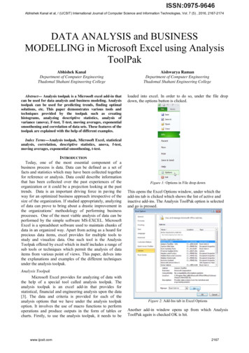
Abhishek Kanal et al, / (IJCSIT) International Journal of Computer Science and Information Technologies, Vol. 7 (5) , 2016, 2167-2174Now, the Analysis ToolPak is loaded and excel is ready toperform analysis of the data. This can be cross checkedwith the presence of the data analysis button under the datatab of the excel window.Figure 3: Data analysis in Data tabIMPLEMENTATIONNow, upon clicking of the data analysis option under thedata tab, the data analysis pop-up window appears allowingto choose from multiple techniques with different criterionsto perform the different types of analysis on the data as perthe need.Figure 5: Histogram dialog boxTo understand the use of this from a practical point ofview, consider an organization which is worried about itslow employee quorum due to health problems. To solvethis, an analysis of the current age scenario at theorganization is made with the help of a histogram. Thefollowing was the result obtained,FrequencyHistogram86420Figure 4: Data analysis dialog box1. HistogramHistogram is an important statistical tool which is agraphical representation of the distribution of numeric dataover a bin range. From a histogram, it is possible to get anestimate of the probability distribution of a continuousvariable. The histogram can depict information about a dataset such as the current state of a particular system alongwith the scope of improvement. Before the optimizations,for a particular system, histograms can be constructed forreferences post optimization. After the optimizations to aparticular system have been made, histograms can beconstructed again and the two histograms, i.e. the onebefore optimization and the one after optimization can becompared to study the improvements made, thediscrepancies which may have crept in during theoptimization and the differences in the level of stability ofthe two systems.To construct a histogram, histogram is selected from thedata analysis window. Now, the histogram window appearson the screen which asks for the necessary fields for theconstruction of the histogram. Specify the values that haveto be studied as the input range, secondly, specify the binrange in accordance to the input range. Select where theoutput would like to be seen by specifying the Output rangeand check the Chart output option.www.ijcsit.comAGEFigure 6: Histogram of age and no. of health problemsUpon studying the above histogram, it was observedthat the employee age is more on the above 40 side,making it obvious to account for the reason of healthproblems. The organization could now make necessaryamendments to recruit more people on the younger side.2. Descriptive StatisticsExcel already provides with the utilities of formulae likesum, difference etc. These formulae could be used forstatistical functions like mean, median etc. by combiningthe results produced by the different formulae. However,Excel provides for a simpler and faster way to performthese functions. They are called descriptive statistics andfall under the data analysis option under the data tab.Descriptive statistics are a set of terminologies thatsummarize a given set of data along with measures ofdistributiveness or dispersion. However, it must beunderstood that the descriptive statistics are justdescriptive in nature and do not involve generalizationafter a certain limit.2168
Abhishek Kanal et al, / (IJCSIT) International Journal of Computer Science and Information Technologies, Vol. 7 (5) , 2016, 2167-2174which the members of the age data set differ fromthe mean.f. Sample Varianceg. Kurtosis: It depicts whether the data is heavy-tailedor light-tailed.h. Skewness: It is the measure of symmetry or the lackof symmetry of a data set.i. Range: It points to the range of the data set overwhich the values are spread.j. Maximum: Largest value of age in the data set.k. Minimum: Least value of age in the data set.l. Sum: The addition of all the ages.m. Count: The number of ages in the data set.Figure 7: Descriptive statistics dialog boxThe column or data set to be analyzed is specified in theinput range. The output range points to the location wherethe output has to be specified, and the summary statisticsneeds to be checked.To understand this in practical sense, we shall considerthe same situation as the previous one where anorganization is looking at analyzing the age of a sample setof its employees and in the process obtain the descriptivestatistics.MeanStandard ErrorMedianModeStandard DeviationSample 683380139‐0.56270194730255587320Table 1: Descriptive statistics of Age of employeesThe above table provides a general description of thedata set of age of the employees.a. Mean: It depicts the average age of the employees.b. Standard Error: It points to the expected error in themean if we consider other samples from the samepopulation.c. Median: It renders the middle value of the age of theemployees.d. Mode: It gives the value of the age which occurs themost number of times in the given data set.e. Standard Deviation: This expresses the amount bywww.ijcsit.com3. ANOVAThere are often situations involved with data, wheredifferent set of data are exposed to different set ofconditions and then their means need to be checked ifthey are equal. A null hypothesis is proposed anddepending upon the output of the Anova, this hypothesiscan be accepted or rejected. This could be understoodbetter with the help of an example of a hospital whichneeds to carry out some research on the effects of a newdrug in the market and another drug which it used earlierfor the same medical purposes. In this situation, the nullhypothesis would be the fact that when the two types ofdrugs were used on two different set of patients and theyproduced similar results for both the set of patients. Onthe other hand, the null hypothesis would be rejected ifthey produced different results.Thus, in these cases where the means of the differentgroups of the same data need to be studied, ANOVA orthe Analysis of Variance is of great help.Excel provides for 3 techniques of ANOVA:1. Anova: Single Factor2. Anova: Two Factor without Replication3. Anova: Two Factor with ReplicationTo understand the difference between the different typesof ANOVA, we shall consider the example of aninternational university which has students admittedlocally as well as globally and from both the genders.Considering a situation where a professor conductsquizzes at three occasions during a semester. Once,before beginning a topic. Second, after the completion ofthe topic. Third, 4 weeks after the completion of thetopic. In this situation, a Single Factor Anova would beuseful is seeing how the performance of the candidatevaries over the course of the topic being taught.Now, if the professor wishes to study the performance oflocal and international students in the same test apartfrom studying their individual performances, then theAnova: Two Factor without Replication comes handy.A third situation, which involves study of the graspingpower of different genders at the different times inaddition to the analysis of individual studentperformances, then it makes sense to make use of Anova:Two factor with Replication.2169
Abhishek Kanal et al, / (IJCSIT) International Journal of Computer Science and Information Technologies, Vol. 7 (5) , 2016, 2167-2174Anova can be implemented by selecting the requiredAnova technique in the data analysis window whichpops up on clicking the data analysis window under thedata tab.Consider, the following sample data.NAMENorah ReslerBecky ChitwoodMagnolia SlettenLavenia DevaulRaelene KincheloeJed FrankoJoella ColomaDonetta HinerSiu KemptonAlison ShuppKym SleeperToshia CancholaAugusta PrincipatoSumiko SeiboldBuena TreacyAdelaide SartinNathanial LagardeHildegard HornickElenore JessMauricio NguyenCorrie MinesQUIZ 1789373649294713888474392678585927659616978QUIZ 2698376869581757985534147909391926265799269QUIZ 36376756685697958954378466170751005747569582Table 2: Quiz scores of studentsTo perform ANOVA, analysis on selecting the anova:single Factor option. We encounter the Anova window.Figure 8: Anova: Single factor dialog boxUpon selecting, the range of the input values whichincludes the scores in the three columns, the location wherewww.ijcsit.comoutput has to be seen and clicking OK, we observe thefollowing.Figure 9: Results of anova: single factorDepending on the values obtained in the ANOVA table,we either accept the hypothesis or reject it. If the value of Fis greater than the value of F CRIT then, we reject thehypothesis, otherwise, accept it. In the case above, we cansee that F F-crit, therefore we accept the hypothesis at aconfidence level of 95% that there is no significantdifference between the means of the different groups.4. F-TestAnother type of analysis that can be performed on the setof data includes the F-test. This test is useful to analyze thedifference in the variances between different data sets. Weinitially propose a hypothesis and then accept or reject it onthe basis of the F and the F-crit values that are obtained.Variance is basically the quality of being divergent ordifferent from the other members of the data set. With thehelp of F-tests, we can compare the variances between twodata sets, thereby studying which one is more diverge innature.To implement, F-test, the F-test option is selection fromthe data analysis window by clicking on the data analysisbutton under the data tab. In the window, which opens up,we enter select the two data sets, specify the output locationand click on OK.The practical application of this test can be elaborated bythe following example.The table consists of ages of a set of male and a set offemale customers of a grocery store.Male101625263037Female179344751Table 3: No. of customers at a grocery store2170
Abhishek Kanal et al, / (IJCSIT) International Journal of Computer Science and Information Technologies, Vol. 7 (5) , 2016, 2167-2174To study the difference of the variances, we implementthe F-test.Figure 10: F-Test dialog boxThe output obtained is as 531.581.611.891.942.022.121.8Table 4: Yearly profits of a companyThe above table gives a relation between the yearnumber (Since the organization started) and the profitsunder by the organization in million dollars.Figure 11: Results of F-TestIn the Moving Average window, we specify the inputrange as the values whose average trend over time has tobe observed. Depending on the interval needed, themoving average graph is shown. For example, for aninterval of 6, the moving average is the average of the 5previous points and the current data point. Therefore, foran interval of 6, we can also conclude that excel will notbe able to calculate the moving average for the first 5data points since they would not be enough, consideringthe interval is 6.It must be taken care of that the Variance of variable 1must be greater than the Variance of variable 2. If not, thenthe two data sets must be swapped. This is because F is aratio of variance of variable 1 to the variance of variable 2.If F F-crit, then we reject the hypothesis otherwise weaccept it. In the above case, we reject the hypothesis thatthe variances of the two age sets do not differ significantlysince 5.099 5.050(F F-critical)5. Moving AveragesA major type of analysis in organizations involves thestudy of some kind of a data over a period of time. Forexample, a company’s average profit study for the last 5years, or any kind of trends which change over time.Another example could be the supply chain organizations,to understand the trend of demands and prepare itself withexpected quantities of goods that are going to be neededwell in advance. To visualize this kind of data in theappropriate way, excel provides for the construction of amoving average chart. The moving average chart depictsthe changes in the trend along with the changes in theaverage as the trends change. Another aspect of the movingaverages is the fact that it is used to smooth out the peaksand valleys to easily recognize trends. To understand themoving averages better, consider the following data,www.ijcsit.comFigure 12: Moving average dialog boxOn similar lines, the charts can be obtained for differentintervals.Below are the moving averages for the same data butintervals of 2, 4 and 6.2171
Abhishek Kanal et al, / (IJCSIT) International Journal of Computer Science and Information Technologies, Vol. 7 (5) , 2016, 2167-2174Figure 13: Moving Average for Interval 81.611.891.942.022.121.8Table 5: Yearly Profits of a companyFigure 14: Moving Average for Interval 4The exponential smoothing window needs to be fed inwith the input range of values, the output location and adamping factor. This concept of damping factor is usefulfor determining the weighing factor for the latest values.The relation between α and damping factor is:Damping factor Smoothing factor (α) 1If we consider a situation where we set the dampingfactor to 0.9, α becomes equal to 0.1. Thereby, giving theprevious data points a relatively smaller weight (0.1) ascompared to the weight of the recent data point (0.9).Figure 15: Moving Average for Interval 2Another important observation to be noticed in case ofmoving averages is the fact that larger the interval is,smother are the valleys and the peaks. This is because,shorter the interval, closer are the moving average points tothe data points. Thus, the moving average is less smooth innature.6. Exponential SmoothingThere exists another technique used to study the averageof trends over times which is called as the exponentialsmoothing. It is very similar to the moving averages. Theonly difference which exists between these two is the factthat exponential weighs the latest trends more than theearlier ones. The moving averages on the other hand, givesall the values an equal weightage. Both of them are highlysimilar because they are interpreted in similar ways and arecommonly used by the technical analysts to smooth outfluctuations. Since Exponential smoothing lays moreemphasis on the recent data than the earlier ones, they aremore reactive towards latest modifications in data whichmakes the results more at par with the recent changes,making it a popular technique among the analysts. If weconsider the same table as specified previously,www.ijcsit.comFigure 16: Exponential Smoothing dialog boxThe output of the chart obtained for the above set ofconditions is:Figure 17: Exponential smoothing chart2172
Abhishek Kanal et al, / (IJCSIT) International Journal of Computer Science and Information Technologies, Vol. 7 (5) , 2016, 2167-2174Yet again, for this technique, it can be observed thatsmaller the value of the damping factor is, more the valleysand peaks are smoothed out.7. T-testThe T-test is quite similar to the anova technique of dataanalysis. The only difference which exists between t-testand the anova is that anova deals with testing for equalmeans among multiple data sets, t-test can perform thecheck only among two data sets. The t-test is used to testthe null hypothesis that the mean of two sets of data are thesame. The aspect here that needs to be kept in mind is thatonly 2 sets of data can be checked for equal means. Apartfrom this, the hypothesis can be accepted or rejected on thebasis of the output obtained by performing the T-test. Thisis on similar lines with the anova. Consider the same set ofdata as mentioned under the Anova subheading but weshall consider the test marks of only two quizzes,considering the constraint of t-tests to work with amaximum of two sets of data.NAMENorah ReslerBecky ChitwoodMagnolia SlettenLavenia DevaulRaelene KincheloeJed FrankoJoella ColomaDonetta HinerSiu KemptonAlison ShuppKym SleeperToshia CancholaAugusta PrincipatoSumiko SeiboldBuena TreacyAdelaide SartinNathanial LagardeHildegard HornickElenore JessMauricio NguyenCorrie MinesQUIZ 1789373649294713888474392678585927659616978QUIZ 2698376869581757985534147909391926265799269Table 6: Quiz scores of students at a UniversityThe T-test window needs to be fed in with the both theinput ranges separately. There exists a hypothesized meandifference field which needs to be filled in with the value 0since the hypothesis we are considering states that there isno significant difference in the means of the two data sets.www.ijcsit.comFigure 18: T-test dialog boxThe output obtained for the above set of conditions:Figure 19: Result of T-testThis technique involves a two-tail test, if t-Stat -tcritical two tail or t Stat t Critical two tail, then, we rejectthe hypothesis. For the case we have considered, thiscondition is not satisfied, therefore, we cannot reject thehypothesis and the difference between the means observedis too small to be considered significant.8. CorrelationOften, there are situations where there is a need tounderstand how are two data sets related to each other. Inother words, when the values of one data set increase, theother data set may increase or decrease. Statistically, thecorrelation factor always varies between -1 and 1. Apractical application of the correlation could be in the fieldof technical stock market analysis where we would want toidentify the correlation between market indicators andspecific stocks. For example, the relation between customerspending and the price of a stock. If customers spend moreon the products of that company, its stock price will rise,and if he customer spending goes down, the stock price willalso decrease. A correlation coefficient of -1 indicatesnegative correlation, which indicates that if the value of onedata set increases, the value of the other data set willdecrease. A correlation coefficient of 1 indicates positivecorrelation, which implies that if the values of one data setis increasing, the values of the other data set also increase.Correlation must not be confused with causation i.e. onedata set is not causing the other. For better understandingon practical purposes, the following data sets are2173
Abhishek Kanal et al, / (IJCSIT) International Journal of Computer Science and Information Technologies, Vol. 7 (5) , 2016, 019000LIMITATIONSEven though MS excel is a convenient tool for dataanalysis, it does have some limitations. It lacks certaintools like boxplots, which are widely used in statisticalanalysis. There is concern over the format of output ofsome specific functions. [1]. Missing values aresometimes handled inconsistently and incorrectly.Different analyses require the data to be arranged invarious ways. If a variety of different tests are to beperformed, data might need to be rearranged multipletimes. Output may be scattered in many differentworksheets, or all over one worksheet and it may beincomplete or may not be properly labelled, increasingpossibility of misidentifying output. It does not maintaina record of what was done to generate the results,making it difficult to document the analysis, or to repeatit at a later time. [2]TIME SINCE DOJ6313624121201736201Table 7: Age, salary and time since date of joining of employeesCONCLUSIONVarious tools and techniques of analysis toolpak wereexplained and demonstrated. Analysis toolpak was usedto create histograms to solve the problem of lowemployee quorum due to health problems, obtain andanalyze descriptive statistics of ages of a sample set ofemployees in an organization, analyze variance betweenset of scores of a test quiz conducted by a universitywhich enrolls both local and global students of bothgenders using anova, F-test and t-test techniques, studychanges in profits of an organization over a period oftime using moving averages, exponential smootheningand study correlation between age and salary ofemployees in an organization.For the data mentioned above, we find out the correlationbetween the three data sets.The correlation window opens up when we select thecorrelation option in the data analysis window.[1][2]Figure 20: Correlation dialog boxThe output obtained according to the conditions givenabove is shown below.[3]REFERENCESManagement Research: Applying the Principles, Susan Rose, NigelSpinks & Ana Isabel Canhoto.Using Excel for Statistical Data Analysis – Caveats, Eva Goldwater,Biostatistics Consulting Center, University of Massachusetts Schoolof Public Health.Excel easy, Analysis toolpak [Online]. Available -toolpak.html.Figure 21: Result of CorrelationThe correlation between age and salary can be referred toas a positive one since the value is approximately 1. Thus,it would be safe to conclude for the organization that withage, the salary of its employees would increase.On the other hand, the correlation between the Timesince date of joining and salary, and between time sincedate of joining and age are approximately 0.3, whichclearly indicates that there is little or no correlationbetween these fields.www.ijcsit.com2174
under the analysis toolpak. Analysis Toolpak Microsoft Excel provides for analyzing of data with the help of a special tool called analysis toolpak. The analysis toolpak is an excel add-in that provides for statistical, financial and engineering analysis upon the da