WIXLIB

Factor Analysis ExampleQian-Li XueBiostatistics ProgramHarvard Catalyst The Harvard Clinical & Translational ScienceCenterShort course, October 28, 20161

Example: Frailty§ Frailty is “a biologic syndrome of decreasedreserve and resistance to stressors, resultingfrom cumulative declines across multiplephysiologic systems, and causing vulnerability toadverse outcomes” (Fried et al. 2001)§ Common phenotypes of “frailty” in geriatricsinclude “weakness, fatigue, weight loss,decreased balance, low levels of physicalactivity, slowed motor processing andperformance, social withdrawal, mild cognitivechanges, and increased vulnerability tostressors” (Walston et al. 2006)2

Example: FrailtyManifest Variables of Frailty:Body composition:Arm circumferenceTricep skinfold thicknessBody mass indexSlowed motor processing and performance:Speed of fast walkSpeed of Pegboard testSpeed of usual walkTime to do chair standsMuscle Strength:Grip strengthKnee extensionHip extension3

Recap of Basic Characteristics ofExploratory Factor Analysis (EFA)§ Most EFA extract orthogonal factors, which maynot be a reasonable assumption§ Distinction between common and uniquevariances§ EFA is underidentified (i.e. no unique solution)§ Remember rotation? Equally good fit with differentrotations!§ All measures are related to each factor4

Major steps in EFA1.2.3.4.5.6.Data collection and preparationChoose number of factors to extractExtracting initial factorsRotation to a final solutionModel diagnosis/refinementDerivation of factor scales to beused in further analysis5

Step 1. Data collection and preparationv v Factor analysis is totally dependent oncorrelations between variables.Factor analysis summarizes correlationstructurev .vF .Fv1 .vkO1.On1kv1.vkCorrelationMatrixData Matrixv1.vk1jFactor patternMatrix6

Example: Frailty(N 547)Observed Data Correlation Matrixbmiarm skin grip kneehip uslwalk fastwk ------------------------------------bmi 1.00arm 0.89 1.00skin 0.65 0.72 1.00grip 0.25 0.32 0.23 1.00knee -0.41 -0.36 -0.12 0.01 1.00hip -0.34 -0.34 -0.10 0.00 0.62 1.00uslwalk -0.11 -0.03 0.09 0.14 0.26 0.121.00fastwk -0.10 0.01 0.13 0.17 0.29 0.150.891.00chrstand 0.04 0.02 -0.08 -0.09 -0.26 -0.14-0.41 -0.411.00peg 0.05 0.10 0.18 0.24 0.13 0.080.330.35-0.29 ------------------------7

Step 2. Choose number of factorsv Intuitively: The number of uncorrelated constructsthat are jointly measured by the Y’s.v Only useful if number of factors is less than numberof Y’s (recall “data reduction”).v Estimability: Is there enough information in the datato estimate all of the parameters in the factoranalysis? May be constrained to a certain numberof factors.8

Step 2. Choosing number of factorsUse Principal Components Analysis (PCA) to help decide§ Similar to “factor” analysis, but conceptually quitedifferent!§ number of “factors” is equivalent to number of variables§ each “factor” or principal component is a weightedcombination of the input variables Y1 . Yn:P1 a11Y1 a12Y2 . a1nYn§ Principal components ARE NOT latent variable§ Does not differentiate between common and uniquevariances9

Choosing Number of Factors/* Principal Components analysis */Proc factor data frailty METHOD PRINoutstat abc.pca allplots (scree);var bmi arm skin grip knee hip uslwalkfastwk chrstand peg;%parallel(data frailty, niter 1000,statistic Median);run;10

SAS PCA OutputEigenvalues of the Correlation Matrix: Total 10 Average 0.00991.000011

Step 2. Choosing number of factors§ To select how many factors to use, evaluate eigenvaluesfrom PCA§ Two interpretations:§ eigenvalue equivalent number of variables which the factor represents§ eigenvalue amount of variance in the data described by the factor.§ Criteria to go by:§ § § § § number of eigenvalues 1 (Kaiser-Guttman Criterion)scree plotparallel analysis% variance explainedcomprehensibility12

Choosing Number of Factors13

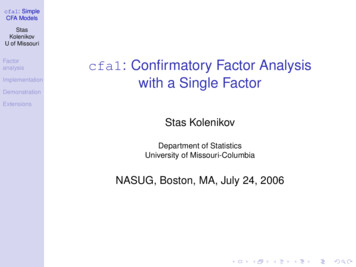
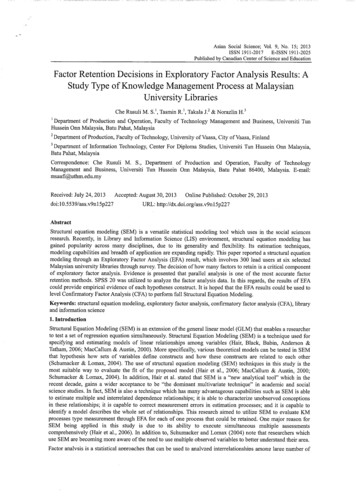
Parallel Analysis(Hayton, Allen, & Scarpello (2004)§ Eigenvalues (EV) that would be expected from randomdata are compared to those produced by the data§ If EV(random data) EV(real data), the derived factorsare mostly random noise§ How to do this in df§ How to do this in STATAType “findit fapara” in STATA to locate the program for free ta/faq/parallel.htm14

Choosing Number of Factors15

Accuracy of Retention Criteria§ EV 1§ Tends to always over estimate number of factor§ Accuracy increase with small number variables &communalities are high§ Scree Test§ More accurate than EV 1§ Subjective and sometimes ambiguous§ Parallel Test§ Most accurate§ Becoming the standard16

Step 3. Extracting initial factors Using MLEProc factor data frailty METHOD MLpriors smc msa residualrotate varimax reorderoutstat abc.fa allplots (scree initloadings loadings);var bmi arm skin grip knee hip uslwalkfastwk chrstand peg;run;17

Step 3. Extracting initial factors Using MLEFactor Pattern l Communality Estimates and VariableWeightsTotal Communality: Weighted 48.803523Unweighted 51.28482431.190521518

Step 4. Factor Rotation§ Steps 2 and 3 determines the minimum numberof factors needed to account for observedcorrelations§ After obtaining initial orthogonal factors, we wantto find more easily interpretable factors viarotations§ While keeping the number of factors andcommunalities of Ys fixed!!!§ Rotation does NOT improve fit!19

Step 4. Factor Rotation§ All solutions are relatively the same§ Goal is simple structure§ Most construct validation assumes simple(typically rotated) structure.§ Rotation does NOT improve fit!20

Step 4. Factor Rotation (Varimax)Factor Pattern ted Factor Pattern 4430.081460.032920.10317-0.186880.779710.7288121

Step 4. Factor Rotation22

Step 4. Factor Rotation (Promax)Promax Rotated Factor Pattern Rotated Factor Pattern r-Factor 0.399170.271831.0000023

Step 4. Factor Rotation (Promax)VarimaxPromax24

Pattern vs. Structure MatrixPromax Rotated Factor Pattern Factor Structure 0925

Step 5. Model Diagnostics:Goodness-of-FitSignificance Tests Based on 547 ObservationsTestDFChi-SquarePr ChiSqH0: No common factors452875.6589 .00011845.17330.0004HA: At least one common factorH0: 3 Factors are sufficientHA: More factors are needed26

Step 5. Model Diagnostics:Residual CorrelationsResidual Correlations With Uniqueness on the Diagonalbmiarmskingripkneebmi0.16866 -0.00004 0.00437 -0.01782 -0.01083arm-0.00004 0.04294 -0.00055 0.00649 0.00358skin0.00437 -0.00055 0.41451 -0.04196 -0.00979grip-0.01782 0.00649 -0.04196 0.85577 -0.00439knee-0.01083 0.00358 -0.00979 -0.00439 0.30444hip0.01499 -0.00468 0.01556 0.00224 0.00151uslwalk0.00359 -0.00047 -0.00157 -0.00833 0.00177fastwk-0.00355 0.00071 0.00134 0.00163 -0.00199chrstand -0.02409 0.00652 -0.00236 0.00008 -0.01761peg-0.00339 -0.00528 0.03339 0.12758 630.84000Root Mean Square Off-Diagonal Residuals: Overall ndpeg0.0120016 0.0040602 0.0189818 0.0453301 0.0104969 0.0130721 0.0047294 0.0035657 0.0397855 0.057976827

Step 5. Model Diagnostics:Partial CorrelationsPartial Correlations Controlling t Mean Square Off-Diagonal Partials: Overall ndpeg0.0389504 0.0247436 0.0344066 0.0593939 0.0284948 0.0312691 0.0172065 0.0159428 0.0575833 0.0731338353915689528

Step 6. Model Refinement:Analysis of Cronbach Alpha/* Cronbach Alpha */proc corr data frailty nomiss alpha plots;var grip knee hip;run;proc corr data frailty nomiss alpha plots;var uslwalk fastwk chrstand2 peg;run;29

Step 6. Model Refinement:Item Deletion?Cronbach Coefficient AlphaCronbach Coefficient ach Coefficient Alpha with Deleted VariableCronbach Coefficient Alpha with Deleted VariableDeletedVariableDeletedVariableRaw VariablesStandardized VariablesCorr.with TotalAlphaCorr.with aw VariablesStandardized VariablesCorr.with TotalCorr.with 1peg0.3499410.6499590.3171860.526887Uniqueness of Grip 0.85577Uniqueness of Chair Stand 0.7782730

Step 7. Derivation of Factor Scores§ Each object (e.g. each person) gets a factor score for each factor:§ The factors themselves are variables§ “Object’s” score is weighted combination of scores on inputvariablesˆ ˆˆF WY , where W is the weight matrix.These weights are NOT the factor loadings!Different approaches exist for estimating Ŵ (e.g. regression method)Factor scores are not uniqueUsing factors scores instead of factor indicators can reducemeasurement error, but does NOT remove it.§ Therefore, using factor scores as predictors in conventionalregressions leads to inconsistent coefficient estimators!§ § § § 31

Step 7. Derivation of Factor ScoresProc factor data frailty method ML score outstat factpriors smc msa residualrotate varimax reorderoutstat abc.fa allplots (scree initloadings loadings);var bmi arm skin grip knee hip uslwalk fastwk chrstandpeg;run;/* Calculate factor scores */proc score data frailty score fact out abc.scores;var bmi arm skin grip knee hip uslwalk fastwk chrstandpeg;run;32

Exploratory vs. ConfirmatoryFactor Analysis§ Exploratory:§ summarize data§ describe correlation structure between variables§ generate hypotheses§ Confirmatory§ Testing correlated measurement errors§ Redundancy test of one-factor vs. multi-factor models§ Measurement invariance test comparing a modelacross groups§ Orthogonality tests33

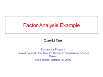
CFA: Conceptual ModelMotorProcessing/SepeedUsual WalkFast WalkPegboardMuscleStrengthHip StrengthKnee StrengthArm CircumferenceBodyCompositionSkinfold ThicknessBMI34

SAS Code/* Confirmatory factor analysis */proc calis data frailty modification;factorBody Factor--- bmi arm skin load1-load3,Speed Factor --- uslwalk fastwk peg load4load6,Strength Factor --- knee hip load7-load8;pvarBody Factor Speed Factor Strength Factor 3*1;covBody Factor Speed Factor 0.;run;35

SAS Output: Standardized Loadings36

SAS Output: Factor Correlations37

Model Fit Statistics§ Goodness-of-fit tests based on predicted vs. observed covariances:1. χ2 tests§ § § § § d.f. (# non-redundant components in S) – (# unknown parameters in the model) Null hypothesis: lack of significant difference between Σ(θ) and SSensitive to sample sizeSensitive to the assumption of multivariate normalityχ2 tests for difference between NESTED models2. Root Mean Square Error of Approximation (RMSEA)§ § § § A population index, insensitive to sample sizeTest a null hypothesis of poor fitAvailability of confidence interval 0.10 “good”, 0.05 “very good” (Steiger, 1989, p.81)3. Standardized Root Mean Residual (SRMR)§ § Squared root of the mean of the squared standardized residualsSRMR 0 indicates “perfect” fit, .05 “good” fit, .08 adequate fit38

Model Fit StatisticsGoodness-of-fit tests comparing the given model with analternative modelComparative Fit Index (CFI; Bentler 1989)§ 1.§ § § 2.The Tucker-Lewis Index (TLI) or Non-Normed Fit Index (NNFI)§ § § compares the existing model fit with a null model which assumesuncorrelated variables in the model (i.e. the "independence model")Interpretation: CFI 100 % of the covariation in the data can beexplained by the given modelCFI ranges from 0 to 1, with 1 indicating a very good fit; acceptable fitif CFI 0.9Relatively independent of sample size (Marsh et al. 1988, 1996)NNFI .95 indicates a good model fit, 0.9 poor fitMore about these later39

Model Fit AssessmentFit SummaryAbsolute IndexFit Function0.2061Chi-Square112.5261Chi-Square DFPr Chi-Square .0001Standardized RMR (SRMR)0.0647Goodness of Fit Index (GFI)0.9527Adjusted GFI (AGFI)0.9054Parsimonious GFI0.6125RMSEA Estimate0.0981RMSEA Lower 90% Confidence Limit0.0812RMSEA Upper 90% Confidence Limit0.1158Akaike Information Criterion148.5261Schwarz Bayesian Criterion226.0061Parsimony IndexIncremental Index18Bentler Comparative Fit Index0.9640Bentler-Bonett NFI0.9577Bentler-Bonett Non-normed Index0.944140