Transcription
Data Fusion with 9 Degrees of Freedom Inertial Measurement Unit ToDetermine Object’s OrientationByLong TranSenior ProjectElectrical Engineering DepartmentCalifornia Polytechnic State UniversitySan Luis ObispoJune 2017
AbstractData fusion is a technique to integrate different types of data to a single unit to provide amore reliable representation of tracking measurement. Today, data fusion can be found in manyapplications such as tracking and surveillance system as well as on mobile applications. In thisproject, 9 Degrees of Freedom (DOF) Inertial Measurement Unit (IMU) composed of 3-axisMagnetometer, 3-axis Accelerometer, and 3-axis Gyroscope are processed to yield the object’srotations in 3 dimensions. While the magnetometer (compass) is used to determine the headingangle, accelerometer is used to determine tilt axis, gyroscope can be process to calculate theangular velocity. Each sensor has its own advantages under different static or dynamic scenarios.By analyzing each sensor separately, the angle output computed from each sensor is then fusedwith angles from other sensors using filter algorithms. For data integration, Complimentary Filterand Extended Kalman Filter Algorithms are used in this project. To achieve a low cost solutionto determine the object’s orientation, the whole experiment is conducted using an Arduino Unoboard integrating with ROHM- sensor shield for Arduino (SENSORSHLD1-EVK-101) thatincludes 9 degrees of freedom.2
Table of ContentsAbstract. 2I.Introduction . 5II. Objective . 6III.Axis and rotation’s definition . 7IV.Type of sensors and their features . 8V.1.Accelerometer . 102.Magnetometer . 123.Gyroscope . 13Fusion method . 151.Complimentary Filter . 162.Kalman filter . 17VI.Data and Analysis . 23VII.Conclusion . 28VIII. Future Works . 291.Compensate misalignment error among 9 DOF axes . 292.Implement different filter models . 29Appendices . 313
Table of FiguresFIGURE 1: RIGHT HAND RULE . 7FIGURE 2: POSITIVE ANGLE DEFINITION . 8FIGURE 3: ACCELEROMETER AX AY AZ 0G . 10FIGURE 4: ACCELEROMETER AX AY 0G, AZ -1G. 10FIGURE 5: AX AZ -0.71G, AY 0G . 11FIGURE 6: EARTH'S MAGNETIC FIELD . 13FIGURE 7: INTERNAL OPERATIONAL VIEW OF A MEMS GYROSCOPE SENSOR. 14FIGURE 8: GYROSCOPE SENSOR . 15FIGURE 9: PROCEDURE'S BLOCK DIAGRAM . 16FIGURE 10: EXTENDED KALMAN FILTER PROCESS . 18FIGURE 11: ROLL ANGLES VS. TIME . 24FIGURE 12: FILTERED DATA (ROLL ANGLES) - ZOOM IN VERSION . 25FIGURE 13: PITCH ANGLES VS. TIME . 26FIGURE 14: YAW ANGLES VS. TIME . 26FIGURE 15: DISPLAY ANGLES WITH AIRPLANE MODEL IN REAL TIME WITHMATLAB (1) . 27FIGURE 16: DISPLAY ANGLES WITH AIRPLANE MODEL IN REAL TIME WITHMATLAB (2) . 28FIGURE 17: EXPERIMENT WITH MULTIPLE SET OF COMPLIMENTARY FILTERS FORROLL ANGLE. 32FIGURE 18: EXPERIMENT WITH MULTIPLE SET OF COMPLIMENTARY FILTERS FORROLL ANGLE (ZOOM-IN). 33FIGURE 19: INTERFACING SENSORSHLD1-EVK-101 WITH ARDUINO . 344
I.IntroductionBefore doing this project, I always think why people need to find multiple solutions to solvea single problem, why not use those extra time to solve other problems rather than going aroundin the same circle. My mind has changed after this data fusion project. Understanding theadvantages and disadvantages between different techniques, I fall in love with this project notonly because it extends my technical knowledge, but also teaches me a new strategy to live. Datafusion has been used for many years in a lot of applications. It has been applied widely in roboticprojects such as in dynamic control system and environment modelling using appropriate modelsand sensors [1], or to combine GPS and Inertial Navigation Systems for Pedestrians in UrbanArea [2] . In the world today where details matter, data reliability has more and more impacts onmany technologies. A rocket with the inaccuracy of a few mili-degree may not hit the target, agunshot arming with a small inclined angles may injure allies instead of enemies. Therefore,combining data is a very challenging job to provide reliable, trustful measurements forexperiments that require high accuracy. This complicated study used to involve manyprofessional engineers and scientists, but in this paper I will help to deliver this fusionknowledge in such an easy and full of details explanation. Throughout this report, I will startwith each sensor specification, and how to determine heading and tilt angles from three set ofsensors. After that, I will walk you through fusion algorithms including Complimentary andKalman Filter, and finally is my experiment and conclusion.Experiencing the hardship when doing researches, I usually find it consume a lot of time torepeat the research paper experiment due to the lack of detailed instructions. People used toexplain the project in a high level block without spending more time organize their works to givetheir peers a full detail guideline of how to build to project ground up. To avoid the struggles that5
I have overcome, I will not stop at the technique to fuse data, I will also walk you through eachstep to rebuild the whole experiment interacting with Arduino C code, Matlab imagerepresentation, as well as the communication to those chip sensors. In the end, I hope you willenjoy my paper and withdraw some good information to expand this project to be bigger andmaybe apply to more useful projects.II.ObjectiveThe purpose for this project is to design a low cost Inertial Measurement Unit via SensorFusion Algorithms in Arduino Environment to utilize sensor data to and optimize the solution ofdetermining the object’s orientation. Three types of sensors are used: Accelerometer, Gyroscopeand Magnetometer to form a 9 Degrees of Freedom are fed to two different filter systemsincluding Complimentary and Kalman Filter to reduce the sum of square error and be able toreact on both dynamic and static system. Without any initial setup information, the system is ableto determine the shape and angles in full 3D – 360 degrees on each axis.6
III.Axis and rotation’s definitionBefore going further to details, let’s define the reference for three sensors and their rotationaxis. Based on the right hand rule, and its representation of axis and positive rotation definition:The pointing direction of your index finger is in the direction of X.Now curl your middle finger to point toward the Y’s direction.Lastly raise your thumb up, that is Z’s directionFigure 1: Right hand ruleNow, the positive rotation is defined as when the object rotates clockwise around each axis lookfrom the origin toward the positive direction.Rotate clockwise around x-axis, that is roll ( ).Rotate clockwise around y-axis, that is pitch ( ).Rotate clockwise around z-axis, that is yaw ( ).7
Figure 2: Positive Angle DefinitionIV.Type of sensors and their featuresThree type of sensors: Accelerometer, Gyroscope, and Magnetometer will be covered in thissection. Each come with their advantages and disadvantages in the method of how to calculatethe roll ( )– pitch ( ) – yaw ( ) angles using each sensor. For the simplicity of the project, Ibought the ROHM- sensor shield for Arduino (SENSORSHLD1-EVK-101) that includes 9degrees of freedom (DOF). The module consists of an accelerometer (KX122), a gyroscope(KXG03), a magnetometer (BM1422), an analog temperature sensor (BDE0600G), a digitalbarometric pressure sensor (BM1383GLV), a hall switch sensor (BU52014HFV), an analog UVsensor (ML8511), a digital color sensor (BH1745), an optical proximity sensors and ambientlight sensor (RPR-0521). For the scope of this project, we only use the accelerometer, gyroscopeand magnetometer sensor, all three sensors are mounted onto the sensor shield, so we don’t haveto worry too much about the alignment errors among the 9 axes. Note that, if you buy the threesensors separately, you need to aligns your sensors in such a way that each three axes (XYZ) ofeach sensor matches with other XYZ axis from other sensors. The specification ofSENSORSHLD1-EVK-101 unit is showed in Table 1.8
Table 1: SENSORSHLD1-EVK-101 specificationPower RequirementInput Voltage3.3 – 5 VDCPower1.2 W maxMeasurementAccelerometer (KX122)Range 2g, 4g, 8gResolution16 bits (65536)Non – Linearity0.6% of FSNoise0.75 mg RMS at 50 HzOutput Data RateTypical 50 HzGyroscope (KXG03)Range 256, 512, 1024, 2048 deg/sResolution16 bits (65536)Non - Linearity0.5% of FSNoise Density0.03 deg/sec/ HzOutput Data RateUp to 51200 HzMagnetometer (BM1422)Range 1200 TResolution16 bits (65536)Output Data Rate100 Hz9
1. AccelerometerAccording to [3], the accelerometer measures all forces that apply to the object. We couldthink of a ball is floating inside a cubic box. When there is no force applied, the ball will befloating in the center of the box.Figure 3: Accelerometer ax ay az 0gIn the above picture, I also assign the sign to each of the wall in 3 X-Y-Z directions. If weplace this box standstill on Earth, the only force that applied to the box now is the gravitationalforce. We know force is equal to mass multiply with acceleration or F ma.Figure 4: Accelerometer ax ay 0g, az -1g10
This example shows the box get -1g (1 g 9.81 m/s2) on the Z direction. Similarly, it will get1g for each of the direction it faces to the ground.So far, we have analyzed the force measured by the accelerometer on a single axis. In fact,this sensor can measure on 3 degrees of freedom. Let’s take another example where the X and Zcorners are facing down to the ground, and the angle between x and z is 45o degree.Figure 5: ax az -0.71g, ay 0gThe total acceleration for a standstill object on Earth is 1g, or a x2 ay2 az2 1 (g). X and Zis 45 degrees between each other. ax az and ay. 0 2 ax2 1 ax az 0.71g which isequivalent Pythagoreans theory [4].According to the document AN3461 from Freescale Semiconductor [5]: with the three setsof rotation matrices1Rx( ) (0000𝑐𝑜𝑠 𝑠𝑖𝑛 ) 𝑠𝑖𝑛 𝑐𝑜𝑠 𝑐𝑜𝑠 Ry( ) ( 0𝑠𝑖𝑛 010 𝑠𝑖𝑛 cos 0 ) Rz( ) ( 𝑠𝑖𝑛 𝑐𝑜𝑠 0𝑠𝑖𝑛 0𝑐𝑜𝑠 0)01Solving the Rxyz RxRyRz for the pitch and roll angles, we get11
𝑎tan( ) 𝑎𝑦tan( ) 𝑧𝑎𝑥2 𝑎 2 ) (𝑎𝑦𝑧or in Arduino C code:Using the accelerometer alone could not help you to determine the yaw angle. This is dueto the fact that when the z axis is facing down to the ground, no matter what yaw angle yourotate around the z-axis, it always measures az 1g and ax ay 0. Therefore, we need anothersensor to calculate the yaw angle.Accelerometer is very accurate in long term, and the roll and pitch angles can becalculated precisely when the object is standstill on Earth. However, when the sensor is moving,the moving acceleration will impact the rotation calculation. However, if we apply a low passfilter to the output of the accelerometer, most of the noise and the external force acceleration willbe removed, the filtered value is then used to integrate with other sensor which is covered insection [V].2. MagnetometerMagnetometer (compass) is an instrument that measure the magnetic field’s strength in aparticular position. People have used compass for thousands years to determine the heading(yaw) angle. We know that the Earth is like a giant magnet with the two North and South poleson two sides when the Earth spin around itself. When magnetometer is on a flat surface, with noother electro-magnetic field surrounding, the yaw angle is calculated as:12
𝑚 tan 1 (𝑚𝑦)𝑥Note that, this formula is incorrected when the sensor is tilted. I will cover the tiltcompensation later on in the fusion algorithm part [V].When rotate the magnetometer clockwise, the yaw angle should increase, and decreases forthe opposite direction. If you find the opposite, this can be done by changing the sign of your ydirection value. This happens due to the magnetometer is facing upside down.Figure 6: Earth's magnetic field3. GyroscopeGyroscope detects angular velocity based on the microelectromechanical systems(MEMS). A small resonating mass attached to the MEMS is shifted as the angular velocitychanges. Follow Newton’s law of conservation of momentum, the output movement isconverted to a small electronic signal, which is then amplified and read by a controller [6]. Inshort, each gyroscope channel measure angular velocity (rotation speed) around one of theaxis. For this project, we use a full 3 DOF to capture the changes in all three X-Y-Zdirections.13
Figure 7: Internal operational view of a MEMS gyroscope sensorTo go from angular velocity to the rotation angle, the Math can be easily known as:Angle angular velocity * timeOr: * t * t * tWhere , , and are angular velocity of roll ( ), pitch ( ), and yaw ( ) angle respectivelyThe only problem with the gyroscope is its calculation drift overtime because of theintegration. A small error measuring at one time will carry on by the integral. In addition to that,due to the inertia, the gyro – rates won’t come back to zero when object is standstill. Forexample, if the raw data is measured at an value, your object was moved and then put back tothe standstill state, the value measured will be different from . However, gyroscope is veryaccurate in short term. Therefore, people usually apply a high pass filter to the gyroscopemeasurement after they obtain the angular rate from the sensor [7].14
Figure 8: Gyroscope sensorV.Fusion methodIf you read up to this point, you probably already have a basic knowledge of how tocalculate the three roll, pitch, and yaw angle from the accelerometer, gyroscope, andmagnetometer.The first step is to combine the accelerometer and magnetometer to calculate the tiltcompensation for the yaw (heading) angle. According to Jay A. Farrell [8], we will use the rolland pitch values from the calculation of accelerometer in the formula to calculate the headingwith compensation.Mx mx . cos( ) mz . sin( )My mx . sin ( ) . sin ( ) my . cos ( ) – mz . sin ( ) . cos ( )𝑀𝑦 tan 1 𝑀𝑥15
After that, the three angles will be integrated with the three independent angular calculation fromthe gyroscope to form a more accurate result. Below is the whole procedure block diagram:Figure 9: Procedure's block diagramEverything will be the same except for the filter part. In this project, I will useComplimentary filter and Kalman filter to optimize the output angle calculated from eachindividual sensor.1. Complimentary FilterThe name of this filter probably explain for its calculation. It basically takes advantage ofeach sensor and compensate for the disadvantages the other sensors have. In this case, as Ialready explained above, accelerometer performs the best with low frequency while gyroscopeperforms the best with high frequency. Complimentary filter is simple and easy to use, it16
contains a fixed value for low pass and high pass’s weights. In short term, we use data from thegyroscope, and in long term, we use data from accelerometer. The filter has the following form:CF angle HP weight * (CF angle gyro data * t) LP weight * acc dataWhere the two constant HP weight (high-pass weight) and LP weight (low-pass weight) have toadd up to one. From my experiment, HP weight value should be very close to one, andLP weight should be very close to zero. Several experiments are performed with different set ofhigh pass and low pass weights - Appendix B, I visually look at the graph generated from eachmeasurement and compare with accelerometer and gyroscope output in slow motion and highmotion respectively. As a result, Complimentary Filter works the best when HP weight 0.98and LP weight 0.02. The expression becomes:CF angle 0.98 * (CF angle gyro data * t) 0.02 * acc dataThe expression of course is put in an infinite loop with a fix t time constant forsimplicity. Every cycle, the new filtered value is equal 98% of the previous filter-angle valueadding with the angle calculated by gyroscope data, the whole thing adds with 2% of anglecalculated from the accelerometer/magnetometer data. Note that, different weights are used andshown in Error! Reference source not found.Because the two low pass and high pass weights are fixed at the beginning, overtime, thiscomplimentary filter will result in a more drift result, and yield a small inaccuracy in themeasurement. We need a better filter; it is called Kalman filter.2. Kalman filterUnlike the complimentary filter where it uses a fixed number for low pass and high passweight. Kalman filter is an algorithm that takes into account a series of measurements overtime,17
in this case, they are the measurement from all three sensors used in this experiment, with themodel noise and the measurement noise, the filter is able to dynamically calculate and update theweight – or Kalman gain value. This system is heavy in math, but provide a more accurate resultthan those based on single measurement alone.Kalman filter consist two main steps: measurement update, and time updateIn this project, the three roll, pitch and yaw angle are independent; therefore, each anglecould be tracked separately as following:Figure 10: Extended Kalman Filter ProcessAccording to Kristian Sloth Lauszus [9], let’s define: ], ′𝑏xk [𝑄 Q [01A [00] 𝑡,𝑄 ′ 𝑏 𝑡],1H [1 0],B [ 𝑡0]uk-1 ’,𝑃P [ 00𝑃101𝐼 [00]1𝑃01𝐾], and K [ 0 ]𝑃11𝐾1where xk is the state variable consisting two elements: angle and bias angular velocity18
A is the state transition model which is applied to the previous state Xk k-1B is the control input model which is applied to the control vector uk-1H is the observation model which maps the true state space into the observed spaceQ is the covariance of the process noiseR is the covariance of the observation noiseP is the estimate covariance matrixK is the Kalman gainTime Update (Predict) stepStep 1: Xk k-1 A xk-1 k-1 B ’ 𝑏[ ′] [𝑘 𝑘 1 𝑏[ ′]1 𝑡 𝑡][ ] [ ] ′ 𝑏 𝑘 1 𝑘 1010 𝑡 ( ′ ′𝑏 )] ′𝑏𝑘 1 𝑘 1 [𝑘 𝑘 1As you can see, the new angle is equal to the previous old angle plus the difference of anglerate multiply by trate newRate - bias;angle dt * rate;Step 2: Pk k-1 A Pk-1 k-1 AT Qk[𝑃00𝑃10𝑃011 𝑡 𝑃00] [][𝑃11 𝑘 𝑘 1𝑃1001𝑃011][𝑃11 𝑘 1 𝑘 1 𝑡𝑄 0] [010] 𝑡𝑄 ′ 𝑏19
𝑃[ 00𝑃10𝑃 𝑡( 𝑡𝑃11 𝑃01 𝑃10 𝑄 )𝑃01] [ 00𝑃11 𝑘 𝑘 1𝑃10 𝑡𝑃11𝑃01 𝑡𝑃11]𝑃11 𝑄 ′ 𝑏 𝑡The equation can be translated to the Arduino code as following:P[0][0] dt * (dt*P[1][1] - P[0][1] - P[1][0] Q angle);P[0][1] - dt * P[1][1];P[1][0] - dt * P[1][1];P[1][1] Q bias * dt;Measurement Update (Predict) stepStep 1:Define S H Pk k-1 HT R𝑃S [1 0] [ 00𝑃10𝑃011][ ] 𝑅 P00 k k-1 R𝑃11 𝑘 𝑘 1 0S P[0][0] R measure;Kk Pk k-1 HT S-1[𝑃𝐾0] [ 00𝐾1 𝑘𝑃10𝑃011 1][ ] 𝑃11 𝑘 𝑘 1 0 𝑆𝑃[ 00 ]𝑃10 𝑘 𝑘 1𝑆K[0] P[0][0] / S;K[1] P[1][0] / S;20
Step 2:Define yk zk – H xk k-1 𝑦𝑘 𝑧𝑘 [1 0] [ ′ ] 𝑧𝑘 𝑘 𝑘 1 𝑏 𝑘 𝑘 1𝑥𝑘 𝑘 𝑥𝑘 𝑘 1 𝐾𝑘 𝑦𝑘𝐾 𝑦 [ ′] [ 0 ]′] 𝑏 𝑘 𝑘 𝑏 𝑘 𝑘 1𝐾1 𝑦 𝑘[y newAngle - angleangle K[0] * y;bias K[1] * y;Step 3:Pk k-1 (I – Kk H) Pk k-1𝑃[ 00𝑃10𝑃01𝐾1 0] ([] [ 0 ] [1𝑃11 𝑘 𝑘𝐾10 1𝑃[ 00𝑃10𝑃01𝑃] [ 00𝑃11 𝑘 𝑘𝑃10𝑃0]) [𝑃0010𝑃01𝐾𝑃] [ 0 00𝑃11 𝑘 𝑘 1𝐾1 𝑃00𝑃01]𝑃11 𝑘 𝑘 1𝐾0 𝑃01]𝐾1 𝑃01P[0][0] - K[0] * P[0][0];P[0][1] - K[0] * P[0][1];P[1][0] - K[1] * P[0][0];21
P[1][1] - K[1] * P[0][1];The covariance matrix of process noise (Q) in this case is the accelerometer noise and theestimated bias rate. This information is found from the manual of accelerometer and gyroscopethen round up to the close mili-unit. In addition, the covariance of measurement noise (R) isreferred to the variance of the measurement, if it is too high, the filter will react slowly as thenew measurement has more uncertainty, on the other hands, if R is too small, the output resultbecomes noisy as we trust the new measurement of accelerometer too much. Based on theexperiment, the following values are picked for the process and the measurement noise22
Q angle 0.001;Q bias 0.003;R measure 0.03;VI.Data and AnalysisTo run the experiment with the 9 Degrees of Freedom chips integrated with Arduino, weneed to make sure so stay away at least two feet from electronic devices, magnets, or irons toeliminate the electromagnetic field affecting the magnetometer. First, let the chip standstill thenmove it around for a few seconds then keep repeating combination of static and dynamic processuntil having around one minute of data. It is very important to let the chip standstill betweendynamic movements because we will use static moments as our good reference since the externalforce is equal to zero and the accelerometer data can be used to calculate the accurate angles. Alloutput angles from raw data and two filters are logged and plotted .vs time in the three directionsto compare the result. Figure 11 and shows the roll angles of the system using raw data andboth Complimentary and Kalman Filtered data where the blue curve represents the anglecalculated from the accelerometer, the orange curve represents the angle calculated from thegyroscope, and the red and black curves are the result from Kalman filter and Complimentaryfilter respectively. The IMU was keeping static in the first 4 seconds, from 10s to 14s, from 15sto 17s, from 18s to 20.5s, from 21s to 23s, from 24s to 25s, and was moving otherwise.23
Figure 11: Roll Angles vs. TimeThe two problems with gyroscope and accelerometer can easily be observed on this graph.The blue curve (accelerometer) is quite noisy – with a lot of oscillations when the sensor ismoving, but accurate in long term – or when it stays flat. The gyroscope is more accurate in shortterm, but has a drift problem in long term. As you can see, the orange curve diverges and keepsgoing down instead of going back to the same level as before.By fusing the two accelerometer and gyroscope sensors using the Complimentary Filter(black), and the Kalman Filter (red), these two black and red curves show the two filters reducethe oscillation of the acceleration noises, and follow the shape of the gyroscope angles in highlydynamic system. Both filters do a pretty good job, but Kalman filter surely has more impacts onthe result. As I explain in IV-1, angles calculated from accelerometer sensor can be used as areference when the object is not moving; for example, in the first 4 seconds, and from 10s to 14s,both filters are in line with the accelerometer angle. At 14s, the IMU was moving for one second,and holding static for the next two seconds, from what being shown in Figure 11, only the24
Kalman Filter angle align on top of the accelerometer angle, the Complimentary Filtered angletakes two seconds to reach the reference. The same things happen from 18s to 20.5s, from 21s to23s.Let’s look at the zoom-in version in Figure 12Figure 12: Filtered data (roll angles) - zoom in versionThe pitch and yaw angles are plotted in Figure 15 and Figure 16.25
Figure 13: Pitch Angles vs. TimeFigure 14: Yaw Angles vs. Time26
Reading the graph can help us analyze the results, but does not help to observe the data inreal time. In fact, I also wrote a small program in Matlab that communicate with the Arduinoboard and grab data and display with an airplane model in every 100ms. Figure 15 and Figure 16show some examples when the IMU board tilt at certain angles on three turning directions.Figure 15: Display angles with airplane model in real time with Matlab (1)27
Figure 16: Display angles with airplane model in real time with Matlab (2)In all examples above, the airplane always matches the pose of the Inertial MeasurementUnit board. Of course, there is a maximum delay of 100 ms due to the slow update rate of Matlabapplication (10 Hz). However, if the board is rotated slowly, one can observe no difference in thepose between the airplane model and the Arduino board. This can clearly show that ourexperiment is successful. You can check out my demo at: https://youtu.be/Qqu J5i-fMkVII.ConclusionTo summarize, data fusion is used in every day of life to help to achieve the best accuratemeasurement. This project is a good way to show how collaboration will affect the overall result.In the experiment that we involve throughout the report, the gyroscope or accelerator ormagnetometer themselves can determine the rotation angles. However, by combining the full28
IMU with three sensors together, we can actually get a more promising result. I also use the twodifferent type of sensors to differentiate the accuracy between the twos. The complimentary use aconstant weight for both low pass and high pass filter and does not react to the change of theoverall system. On the other hand, the Kalman filter takes into account the historical/statisticalvalue to analyze for the current state; therefore, it can react faster and better. This implies a goodstrategy for those stubborn people who never want to change, they will end up similar to thecomplimentary filter, easy and simple, but not accurate enough. If you already read theintroduction, you now can guess why I fall in love with this project and what strategies Iwithdraw.VIII.Future Works1. Compensate misalignment error among 9 DOF axesThe project assumes perfect alignment among 9 degrees of freedom axes. However, inreality, there is always a small misalignment that decreases the accuracy of the outputangles. My future work includes finding a way to calibrate the chip to compensate for themisalignment error.2. Implement different filter modelsComplimentary and Extended Kalman filter are well known filters that has been used forseveral decades. Besides that, there are also other filter such as fuzzy adaptive federatedKalman Filter (FAFKF) or Extended Information Filter (EIF) that may yield a moreaccurate results.29
Reference[1] B. Siciliano, "Multisensor Data Fusion," Springer Handbook of Robotics, pp. 19-20, 2008.[2] K. B. &. J. Demkowicz, "Data Integration from GPS and Inertial Navigation Systems forPedestrians in Urban Area," TransNav, vol. 7, 2013.[3] G. Gangster, "Accelerometer & Gyro Tutorial," [Online]. meter-Gyro-Tutorial/. [Accessed 2017].[4] T. P. Site, "The Pythagorean Theorem," [Online]. /mathematics/geometry/the-pythagoreantheorem/. [Accessed 2017].[5] MarkPedley, "Tilt Sensing Using a Three-Axis Accelerometer," vol. AN3461, pp. 5-10, 032013.[6] Ronzo, "How a Gyro Works," [Online]. oscope/how-a-gyro-works. [Accessed 2017].[7] J. Esfandyari, "Sensor Technology," [Online]. r solutions mems/. [Accessed 2017].[8] J. A. Farrell, Aided Navigation, McGraw Hill, 2008, pp. 356-357.[9] K. S. Lauszus, "A practical approach to Kalman filter and how to implement it," 10 9 2012.[Onlin
bought the ROHM- sensor shield for Arduino (SENSORSHLD1-EVK-101) that includes 9 degrees of freedom (DOF). The module consists of an accelerometer (KX122), a gyroscope (KXG03), a magnetometer (BM1422), an analog temperature sensor (BDE0600G), a digital barometric pressure sensor (BM1383GLV), a hall switch sensor (BU52014HFV), an analog UV