Transcription
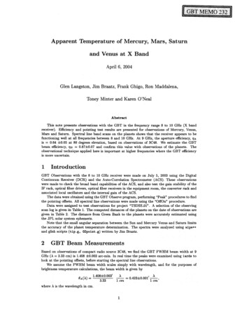
Apparent Temperature of Mercury, Mars, Saturnand Venus at X BandApril 6, 2004Glen Langston, Jim Braatz, Frank Ghigo, Ron Maddalena,Toney Minter and Karen O'NealAbstractThis note presents observations with the GBT in the frequency range 8 to 10 GHz (X bandreceiver). Efficiency and pointing test results are presented for observations of Mercury, Venus,Mars and Saturn. Spectral line band scans on the planets shows that the receiver appears to befunctioning well at all frequencies between 8 and 10 MU. At 9 Gliz, the aperture efficiency, 71Ais 0.64 0.05 at 80 degrees elevation, based on observations of 3C48. We estimate the GBTbeam efficiency, ?T B 0.87 0.07 and confirm this value with observations of the planets. Theobservational technique applied here is important at higher frequencies where the GBT efficiencyis more uncertain.1 IntroductionGBT Observations with the 8 to 10 GHz receiver were made on July 5, 2003 using the DigitalContinuum Receiver (DCR) and the Auto-Correlation Spectrometer (ACS). These observationswere made to check the broad band capabilities of the ACS, and also test the gain stability of theIF rack, optical fiber drivers, optical fiber receivers in the equipment room, the converter rack andassociated local oscillators and the internal gain of the ACS.The data were obtained using the GBT Observe program, performing "Peak" procedures to findthe pointing offsets. All spectral line observations were made using the "OffOn" procedure.Data were assigned to test observations for project "TSDSS 01" . A selection of the observingscan log is given in Table 1. The computed distances of the planets on the date of observations aregiven in Table 2. The distance from Green Bank to the planets were accurately estimated usingthe JPL solar system ephemeris.Note that the small angular separation between the Sun and Mercury Venus and Saturn limitsthe accuracy of the planet temperature determination. The spectra were analyzed using aips and glish scripts (tip.g, GOpoint.g) written by Jim Braatz.2 GET Beam MeasurementsBased on observations of compact radio source 3C48, we find the GBT FWHM beam width at 9GHz (A 3.33 cm) is 1.408 0.003 arc-min. In real time the peaks were examined using iards tolook at the pointing offsets, before starting the spectral line observations.We assume the FWHM beam width scales simply with wavelength and for the purposes ofbrightness temperature calculations, the beam width is given by 1.408 0.003'3.33where A is the wavelength in cm.0A(A)1 CM 0423 0001' A1 cm '
Following Baars (1973) we use the main beam area, urn, formula below, 1.133 OA.At 9 GHz, the GBT beam area is 2.246 arc-min 2 1.900 x 10 -7 s2.1 ACS SetupFor the first hour of the tests, the ACS was set up in the Al 800 MHz bandwidth, three level,dual polarization mode, producing 2048 lags per spectrum. The planets Mars and Venus wereobserved in this mode, stepping by 600 MHz across the receiver band, at 8400, 9000 and 9600 MHzcenter frequencies, covering the frequency range 8000 to 1000 GHz, with 200 MHz overlap betweenspectra. The Cal On/Off switching cycle of 1 Hz was selected, using external blanking and externalCal On/Off signals. The switching signal selector was configured to route the internally generatedACS switching signals back into the ACS. The integration time of 10 seconds was selected. Scandurations were usually 60 seconds.During the second hour, the ACS was set up in the Al,B1,C1,D1 800 MHz mode simultaneouslyobserving 4 center frequencies, 8400, 9000, 9600 and 10200 MHz. Each spectrum was 800 MHzwide, producing 2048 lags per band.2.2 Tipping CurvesNo observations of the system temperature versus elevation angle were made during this observingsession, since the atmospheric attenuation was expected to be small in good weather. Observationsat other times show that a "typical" atmospheric attenuation value of T 0.01 can be assumed ingood weather, when observing at 9 GHz.Figure 1 shows an example a fit of attenuation to an observation at 9 GHz. In this case, theobservations are well fit by attenuation, T0.008 0.001. Other observations in less excellentweather showed tau 0.014. For the remainder of this document T 0.01 is assumed.Table 3 lists the atmospheric attenuation factor, exp(taulsin(E1)) for the elevation angles atthe time of observation of the planets.3 3C48Compact radio source 3C48 is used as a calibration reference for radio wavelength observations inthe frequency range 1.4 to 15 GHz. At 9 GHz, the Ott et cd.(1994) fit yields a flux density of 3.112 0.244 for 3C48. Note that the uncertainty in the 3C48 flux density dominates the our uncertaintyin the measurement of the GBT efficiency.For bright radio sources like 3C48, the dominant observational uncertainty is the uncertainty inthe calibration of the effective temperature of the noise diode values. For 3C48 at 9 GHz we observeTR 5.509 0.009 K and Tr, 5.659 0.012 K. Notice that the RMS noise in the measurements forthe two polarizations is much smaller than the difference between the two values. We assuming littlecircular polarization for source 3C48 and the planets. We adopt the average left and right circularpolarization temperature for antenna temperature and take the difference between the temperatureof the average and the difference of the polarizations as an estimate of the error in the antennatemperature (le. TA [(TR -1- Tr,) (TR —Tr)] 5.584 0.075).Adopting the notation and numerical values of Ghigo et al (2001), the source flux density isS 2kTA11AAgwhere k is Boltzman's constant, and A, is the geometric area of the GBT, 7854 m 2 . Substitutingthe numerical values for k and the 3C48 observations, we findT1A 2761 x 5.584 0.075 13.112 0.244 x 7854 2.845where the major contribution to the uncertainty in271A5.584 0.0753.112 0.244 0.64 0.05,is the uncertainty in the flux density of 3C48.
3.1 Planet Data AnalysisThe four primary conversion factors from observed antenna temperature are summarized below.rIA Aperture efficiency, determined by observations of compact extra-galactic radio sources.BeamDilution The ratio of the telescope beam area to the angular area of the planet on the dateof observation. This is a large factor if the angular size of the planet is much smaller than thetelescope beam.DiskFactor The convolution function of a uniform temperature disk with a Gaussian beam. Thisis a small factor if the angular size of the planet is much smaller than the telescope beam.T Atmospheric attenuation. At 9 GHz in good weather the atmospheric attenuation factor is small,less than 3 percent for these observations.The beam dilution factor is the ratio of the areas of the planet and the GBT beam area atthe frequency of observation. The planet angular area is simply r8 s2 /4, where OS is the angulardiameter of the planet. Table 2 lists the angular sizes of the planets on the date of observations.Following Baars (1973) equation 12, we correct the antenna response for the the disk shapedprojected surface of the planet usingwhere x 0s11.2 OA. Table 3 lists the dilution and disk factors on the date of observations.The conversion from antenna temperature, TA, to brightness temperature, TB requires anestimate of the beam efficiency TIB. We assume the GBT radiation efficiency, 7M, is 0.99 at 9GHz and estimate 7)13 using equation 10 of Baars 1973:-7nAnmAg 0.64 0.05 x 1.9 x 10 x 78542—A0.99 x 0.03332'M?is —The computation of the physical temperature of the planets was performed using aips dishglish scripts. An example script is included in appendix A.3.2 MarsThe 9 GHz band average antenna temperature towards Mars was 5.447 0.075 K. On July 5, 2003,Mars was 8.02 x 10 7 km from Green Bank, and the angular diameter of Mars was 0.290 arc-min.The beam dilution, disk and atmospheric attenuation factors are given in Table 3. Using 77130.87 0.07 yields TB,Mars 221 16 K.Figure 6 shows the antenna temperature of Mars, calibrated by measurement of the intensity ofthe noise diode values, which are toggled on and off at a 1 Hz rate during the scans. Three scansare shown in this figure, one centered at 8400 MHz, one at 9000 MHz and the third at 9600 MHz.Figure 7 shows the same data as figure 6, zoomed on the average antenna temperature of Mars.Notice the undulations in the band pass spectrum which are due to the resonances in the GBTfeed and receiver system. There is a very strong line at 8400 MHz in the Mars spectrum due todown link data from satellites at Mars. This signal is much much stronger in the Right circularpolarization.The orbit of Mars is eccentric, e 0.093, and the physical temperature of Mars is dependenton the distance from the Sun at the time of observation according to the function below (de Pater1990):,x. rTB,mars,Ave(v) TB,Marskli ) \./I'mwhere rm is the mean solar distance, 1.524 AU, and Mars,Ave( V ) is the average temperatureof Mars. At the date of these observations, r 1.402 AU, so the correction factor from observedbrightness temperature to average temperature is 0.959, yielding TB,Mar8,Ave(9G.11Z) 212 15 K.This value is higher than the value reported by Rudy (1987) at 2 cm, 193 10 K, averaged overthe whole Mars disk and corrected to the average temperature at the mean Mars orbital radius.Figure 9 shows the brightness temperature of Mars, calibrated by calculating ri B (u) for eachspectral channel, using the observations of 3C48 at the same frequency. The glish scripts in theT
appendix show the details of this calibration procedure. Notice the narrow features due to theGBT feed and receiver are removed by this calibration process. Figure 10 shows the same data asfigure 9, centered on the average brightness temperature of Mars. The scans centered at 9000 and9600 MHz show good temperature agreement, while the scan at 8400 MHz center frequency has adifferent average brightness temperature where overlapping with the 9000 MHz scan. This may bedue to gain compression due to the strong signal at 8400 GHz.3.3 MercuryThe observations of Mercury were made when the planet was only a few degrees from the Sun andthe spectral baselines show significant undulations. The 9 GHz average antenna temperature was0.59 0.18 K. On July 5, 2003, Mercury was 1.988 x 10 8 km from Green Bank. and the angulardiameter of Mercury was 0.0841 arc-min. The beam dilution, disk and atmospheric attenuationfactors are given in table 3. Using nE, 0.87 0.07 yields TB,Mercury 282 85 K. For Mercurythe uncertainty in the estimate of the effective brightness temperature is dominated by undulationsin the spectral baselines. The accuracy of these observations could be improved by observations ofMercury when its angular distance from the Sun was greater. Figure 6 shows the undulating TBspectrum of Mercury. This figure shows the good agreement in the calibration of the overlappingfrequency range of the four spectra. The undulations of the TB versus frequency happen to bringthe Mercury brightness temperature to a reasonable at 9 GHz, the reference frequency for thisstudy. These observations should be repeated when Mercury is further from the Sun.VLA observations at 6 cm by Burns et al. 1987 show the brightness temperature of Mercuryis significantly greater on the Sun-lit side of Mercury. Klein (1970) finds the Mercury effectivetemperature ranging between 300 and 440 K for the night and day sides respectively.3.4 SaturnThe 9 GHz average antenna temperature towards Saturn was 5.256 0.062 K. On July 5, 2003,Saturn was 1.501 x 10 9 km from Green Bank, and the angular diameter of Saturn was 0.2667 arcmin. The beam dilution, disk and atmospheric attenuation factors are given in table 3. Using na 0.87 0.07 yields TB,Saturn 151.8 12 K.The measurement uncertainty in the estimated brightness temperature is dominated byuncertainty in calibration of the GBT. The observed effective temperature is consistent with thedata of Briggs and Sackett (1989), 165 15 K, that is reported in de Pater (1990).The broad, 200 MHz, undulations in the band spectrum of Saturn near 9800 and 10100 MHzalso appear in the Venus spectra (below), and are likely due to a problem with input spectrometerpower during the observation of 3C48. The 3C48 observation at 10 GHz is used to calibrate theobservations of Venus and Saturn.3.5 VenusThe 9 GHz average antenna temperature was 5.256 0.062 K. On July 5, 2003, Venus was 2.517x 10⁸km from Green Bank, and the angular diameter of Venus was 0.1653 arc-min. The beam dilution,disk and atmospheric attenuation factors are given in table 3. Using 71B 0.87 0.07 yields TB,venus 648 48 K.The measurement uncertainty in the estimated brightness temperature is dominated byuncertainty in calibration of the GBT. Pettengill et al. 1988 measured 636 28 K for the diskaveraged brightness temperature of Venus.Figure 10 shows the brightness temperature of Venus, calibrated by calculating ria (v) for eachspectral channel, using the observations of 3048 at the same frequency. Notice the narrow featuresdue to the GBT feed and receiver are removed by this calibration process. Figure 11 shows thesame data as figure 10, centered on the average brightness temperature of Venus. Notice the veryhigh brightness temperature of Venus, due to the Green house effect. At lower frequencies theatmosphere is more transparent, so that the radio wavelength observations reach deep in the Venusatmosphere, to hotter regions, where the effective temperature is greater.While there is good agreement between frequency bands for the Venus observations, clearly thereis a discrepancy of approximately 20 K where the 800 MHz spectral bands overlap. This differencecorresponds to a 1.5% effect compared to the average brightness temperature of Venus. We have4
examined the glish scripts that are used to produce these spectra, but can find no explanation forthe difference in the equations used to correct for the planet angular size.A possible explanation for the difference in intensities measured for each of the spectral bands isthat the calibration process assumes a single Zy3 value for the reference spectrum for each spectralband. However the system temperature gradually increases with increasing observing frequency.At the low frequency edge of each band the system temperature is over estimated and at the highfrequency edge the system temperature is under estimated. Correcting for this effect would reducethe discrepancies in the overlapping frequency ranges. This model system temperature correctionshould be checked in future tests. The existing software does not easily allow implementing thisThe accurate measurement of the GBT efficiency allows precise measurement of the brightnesstemperature of the planets. These observations show that application of the GBT efficiency beamefficiency, riB , and aperture efficiency, // A , determined from observations of compact radio source3048 yield reasonable results when applied to observations of the planets.If the antenna efficiency factors could be more accurately determined, then more precisemeasurement of the effective temperature of the planets could be made.ReferencesAltenhoff, W. J., Johnston, K. J., Stumpff, P., Webster, W. J. (1994), Astronomy andAstrophysics, vol. 287, no. 2, p. 641-6462. 13aars, J. W. M. (1973) IEEE Trans. Antennas Propagat. AP-21, no 4. 461.3. Briggs, F. H. and Sackett, P. D. (1989), Icarus, Vol 41, 269.4. Burns, J. 0., Gisler, G. R., Borovsky, J. E., Baker, D. N., Zeilik, M. (1987), Nature, Vol 329,234.5. de Pater, Imke (1990), Annual Review of Astronomy and Astrophysics Vol 28, 3476. Ghigo, F., Maddalena, IL, Balser D., and Langston, G. (2001,) "GBT Commissioning Memo:Gain and Efficiency at S-band"7. Klein, M. J. (1970), Radio Science, Vol 5, 397.8. Ott, M. Witzel, A., Quirrenbach, A., Kirchbaum, T.P. Standke, K., J.,Hummel, C.A., (1994) Astronomy and Astrophysics, Vol 284 pg 331.9. Pettengill, J. B., Ford, P. G., Chapman, B. D. 1998, J. Geophys. Res, 92(812): 14,881-92.10. Rao, R., Crutcher, R. M., Plambeck, It. L., and Wright, M. C. H. (1998), ApJ, 502, L75.
Start Stop Object Scan Type Frequency Elevation Start TimeScan Scan(MHz) (d)(UTC)11:05:541Peak8999.999 77.443C4811:09:4683C485Peak8999.999 78.111:14:169103C48OffOn8999.999 78.811:19:0111128999.999 79.63C48OffOn11:22:1914133C48OffOn8999.999 80.111:24:55159600.000 80.5163C48OffOn11:27:209600.000 81.117183C48OffOn11:30:481920OffOn8400.000 81.63C4811:37:092122Mars8400.000 27.4OffOn11:40:01Mars2324OffOn8999.999 27.011:43:04MarsOffOn9600.000 26.6262511:50:192728 VenusOffOn8999.999 29.811:53:182930 VenusOffOn8400.000 30.411:57:20OffOn9600.000 31.23132 Venus12:05:278999.999 32.6OffOn3334 Venus12:08:058999.999 33.336 VenusOffOn3512:11:398999.999 34.0OffOn3738 Venus12:14:578999.999 31.6OffOn40 Saturn3912:18:0442 SaturnOffOn418999.999 32.212:22:49OffOn4344 Saturn8999.999 33.112:26:134546 MercuryOffOn8999.999 26.612:28:114748 MercuryOffOn8999.999 27.112:31:20OffOn4950 Mercury8999.999 27.112:33:17OffOn8999.999 27.452 Mercury5112:35:188999.999 27.8OffOnSun545312:37:418999.999 38.9OffOn5556 Venus12:39:468999.999 39.5OffOn5758 Venus12:47:41OffOn8999.999 79.63C48605913:17:12OffOn8999.834 46.78485 VenusTable 1: Scan Summary of X band observations on 2003 July 5. This observing summary was producedusing the validator program.6
Angular Areaarc-min25.561 x 10-36.603 x 10-22.147 x 10-2116438 1.501 x 10 90.2667 5.586 x 01-2Planet DiameterDistance Angular Size(km)(km)arc-min4866 1.988 x 10 80.08416760 8.015 x 10 70.289912106 2.517 x 10 80.1653SaturnElevation(d)27.127.032.632.2Table 2: Parameters of the Planets used for calculation of the apparent brightness of the planets,including angular size and areas on the day of observation.ObjectNameTR,A(K)(1)(2)Mercury 0.773 0.048Mars 5.371 0.010Venus 5.194 0.017Saturn 3.216 0.020TL,A(K)(3)TA(K)(4)0.413 0.044 0.59 0.185.529 0.011 5.447 0.0755.318 0.018 5.256 0.0623.181 0.015 3.198 0.035Dilution DiskFactor Factor(5)404.434.02104.840.27TB X 91.019245 74192.2 2.6565 12132.1 1.5Table 3: Measured antenna temperatures and computed factors. Column 8 is the brightness temperatureof the planet, excluding the antenna beam efficiency factor, computed from the product of columns 4,5, 6, and 7.
Tip Scan 3 Project TPTCSDSB031 1 10Opacity 0.009 /— 0.000RX temp - 17.405 /— 0.005Tatm 260.000 /— 0.000 2.660TcalSky temperature (K)Fit20604080Elevation (deg)Figure 1: Tipping observations at 9.0 GHz fit to a secant(z) opacity model, whereassumed.8Tatmosphere 260 is
2 : 0 : 3048 : RA; 3048 : RACtr: —0.016Wid: 1.397" Hgt: 5.459dAz:0.0070.014dEl:Tsys: 27.512 -—10100dAz:0.042dB: 0.082Tsys: 27.546 Pass: TCtr: —0.092Wid: 1.406- Hgt: 5.409—100Offset (min)10Offset (min)Figure 2: Pair of Peak scans in the RA direction towards 3C48.7 : 0 : 3048 : Dec11111,1: 3048 . Dec1Ctr: 0.025Wid: 1.411- Hgt: 5.454dAz:dEl:Tsys:—0.0220.01227.554 -Ctr: —0.048Wid: 1.447Hgt: 5.498dAz:0.042—0.023dEl:Tsys: 27.563Pass: TC 1—10—50Offset (min)50Offset (mm)Figure 3: Pair of Peak scans in the Dec direction twoards 3C48.
CN09.58.510TOPO Frequency (GHz)Figure 4: Antenna Temperature versus frequency plot for three pairs of OffOn scans towards calibrationsource 3C48. The antenna temperature is calibrated by measurement of the calibration noise diodeintensity, which is toggled on and off at a 1 Hz rate during the observations.9.58.510TOPO Frequency (0I-1z)Figure 5: Antenna Temperature versus frequency plot for three pairs of OffOn scans towards calibrationsource 3048. Same as previous figure except the temperature range is centered on the average 3C48temperature. Although the radio spectrum of 3C48 is expected to be very smooth, a number of narrowfeatures are seen in the spectrum. These features are due to properties of the feed and receiver system.10
cna)8.59.5TOPO Frequency (GHz)Figure 6: Antenna Temperature versus frequency plot for three pairs of OffOn scans towards planetMars. The antenna temperature is calibrated by measurement of the calibration noise diode intensity,which is toggled on and off at a 1 Hz rate during the observations.TOPO Frequency (GHz)Figure 7: Antenna Temperature versus frequency plot for three pairs of OffOn scans towards planetMars. Same as previous figure except the temperature range is centered on the average Marstemperature. Although the radio spectrum of Mars is expected to be very smooth, a number of narrowfeatures are seen in the spectrum. These features are due to properties of the feed and receiver system.11
098.59.5TOPO Frequency (GHz)Figure 8: Brightness Temperature versus frequency plot for three pairs of OffOn scans towardsplanet Mars. The antenna temperature is converted to brightness temperature by the applicationof measurements of source 3C48, described in the text.(f)0(1.)C CN0CN0C\100(\ITOPO Frequency (GHz)Figure 9: Brightness Temperature versus frequency plot for three pairs of OffOn scans towardsplanet Mars. Same as previous figure except the temperature range is centered on the average Marstemperature. Notice this calibration process removes the sharp features in the Mars spectrum due tothe GBT feed and receiver system.12
0Q)L9I10TOPO Frequency (GHz)Figure 10: Brightness Temperature versus frequency plot in 4 spectral bands for planet Mercury. Theundulations in the spectrum are due to sidelobes of the Sun.13
'8.599.510TOPO Frequency (GHz)Figure 11: Brightness Temperature versus frequency plot in 4 spectral bands for planet Saturn. Thehigh frequency undulations in the spectrum are due to effects of the Sun in the sidelobes.000V-LC)8.599.510TOPO Frequency (GHz)Figure 12: Brightness Temperature versus frequency plot in 4 spectral bans for planet Saturn. Sameas previous figure, centered on the average brightness temperature of the planet.14
TOPO Frequency (GHz)Figure 13. Brightness Temperature versus frequency plot in 4 spectral bands for planet Venus. Thehigh frequency undulations in the spectrum are due to effects of the Sun in the sid.elobes.910TOPO Frequency (GHz)Figure 14: Brightness Temperature versus frequency plot in 4 spectral bans for planet Venus. Same asprevious figure, centered on the average brightness temperature of the planet.15
CasiiScript: ntaxErannp.g.Glish scripts are used to generate the physical temperature plots for the planets based onobservations of calibration sources (glish scripts for calibration of these observations are availableon-line at http://www.gb.nrao.eduk-- , glangsto/gbt/x). An example Glish script is shown below:*script to calculate brightness temperature of Mars as function of frequency*HISTORY# 040302 GIL clean up comments# 040301 GIL attempt correction of \eta B# 040226 GIL update constants# 040217 GIL re-order and compute Temp for 3 frequency bands# 040212 GIL fix glish errors# 040202 GIL change in filler from SPECTROEMTER TO ACS# 031010 GIL add comments, make function physicalTemp()# 030801 GIL initial version for summer school# The observations were performed at C band, with 4 banks of 800 MHz each# scan for calibration (3C48 9 GHz)scanCal : 13# scan with sourcescanSrc : 25(Mars 9 GHz)dataName : '/home/archive/test-data/tape-0001/TSDSS 01'print 'About to import data.'d. import( dataName„,scanCal,scanSrc 1);# speed of light in misecc : 299792458# boltzman's constantk : 1.38 * 10 - -23# utilities needed to do the calculationsinclude '/users/glangsto/flareGlish/ott.g'include '/users/glangsto/flareGlish/polAvg.g'include '/users/glangsto/flareGlish/reducelB.g'orbital radiusdiameter: 1391900SunKm: 1391900 ; SunOrbitKmMercuryKm : 4866 ; MercuryOrbitKm : 57950000VenusKm : 12106 ; VenusOrbitKm : 108110000EarthKm : 12742 ; EarthOrbitKm : 149570000: 227840000: 6760 ; MarsOrbitKmMarsKmJupiterKm : 139516; JupiterOrbitKm : 778140000SaturnKm : 116438; SaturnOrbitKm : 1427000000UranusKm : 46940 ; UranusOrbitKm : 2870300000NeptuneKm : 45432 ; NeptuneOrbitKm : 4499900000PlutoKm : 2274 ; PlutoOrbitKm : 5913000000#distances to the planets on this day; from orbitPlanetseconds#03JUL05 16h00m00 663.066 6h59m20 24d07'03" Mercury#03JUL05 16h00m00 839.672 6h04m58 23d21'54" Venus1.256 11h50m47 5d46'20" Moon#033UL05 16h00m00#033UL05 16h00m00 267.351 22h40m28 -13d20'44" Mars#03JUL05 16h00m00 3070.178 9h26m08 15d56'04" Jupiter#03JUL05 16h00m00 5006.668 6h17m41 22d35'24" Saturn#03JUL05 16h00m00 9655.915 22h19m03 -11d18'23" Uranus#03JUL05 16h00m00 14566.165 21h00m04 -17d01'56" Neptune#03JUL05 16h00m00 14848.257 17h11m04 -13d28'15" PlutodiameterKm : MarsKm#diameter of mars (km)16
*distance to mars (seconds)distanceS : 2 6 7.35 1distanceKm : distanceS c/1000.*distance to planet (km)*get calibration source parameterscalSdRec : polAvg( d.getscan(scanCal))d.plotscan(calSdRec)calTemps: getData(calSdRec): getFreq(calSdRec)calFreqsnChannels: length( calTemps);centerFreq : mbda: 0.01tauetaR: 0.99: 0.000171539002Kmkg: 7854* now examine* vector arrays end in 's'*******get center freq MHzwavelength in cmatmospheric attenuationradiation efficiencyconversion factor for main beam sizele: OmegaM Km * (lambda/m) 2Geometric area of the GBT (m-2)#function to s owthe scale p arameters for Phy sical temp calculationshshowFactors : functio n (centerLambda, diameterKm, distanceKm, srcE1)global x, K, omegaM, thetaS, srcArea, thetaSArcMinthetaS diameterKmidistanceKm * angular size Oraxijiluu0theta ArcMinSthetaS * ((180*60)/Pi)it angular area of planet (sr)srcArea : thetaS*thetaS * pi/4.* gbt FWHM in arcminthetaArcMin : 0.423 * centerLambdathetaA: thetaArcMin / ((180*60)/pi) St angle in radiansprint ": thetaS / (1.2 * thetaA): x*x / 1- exp( -x*x))basis 1973 eq. 12.basis 1973 eq. 12print 'For wavelength centerLambda, ' cm29.97/centerLambda, ' MHz'print 'For frequency print 'Beam FWHMthetaArcMin, 'Arc Min'thetaSArcMin, 'Arc Min'print 'Src Size omegaM: 1.133 * thetaA * thetaAprint 'Dilution Factorprint 'DiskFactor omegaM/ srcAreaKprint 'Assuming atmospheric attenuation ', tau, ' tau at El ',srcEl,'print ' atmospheric correction exp( tau/sin(srcEl*pi/180.))print "return T;* end of showFactors()showFactors( centerLambda, diameterKm, distanceKm, srcE1 27)*function to convert source antenna temp to brightness TemperaturephysicalTemp : function( scanCal, scanSrc, srcArea){ * for debugging, make variables globalglobal calSdRec, srcSdRec, srcSdRecPhysTemp, sd, srcTemps, etaBsglobal is, Ks, thetais, tauFactor, srcEl, omegaBs, calFluxs, calTempsglobal lambdascalSdRec2 : reduceSR( scanCal 1, scanCal) * Calibrate cal (Assume Off On17
# produce a polarization average Single dish recordcalSdRec : polAvg( calSdRec2)# now examined.plotscan(calSdRec)# vector arrays end incalTemps : getData(calSdRec)calFreqs : getFreq(calSdRec)nChannels : length( calTemps);endChannels : nChannels/128# get the calibration source namecalSourceName : calSdRec.other.gbt go.OBJECTcalFluxs : ottFlux(calSourceName, calFreqs): calSdRec.header.azel.ml .valuecalE1lambdas : (c*10 - -6)/calFreqs# convert freq (MHz) to mthetaAs : 0.423 * lambdas * 100. / (180*60/pi) # angle in radians# beam areasomegaBs : 1.133*thetaAs*thetaAs# basis 1973 eq. 12.: thetaS / (1.2 * thetaAs)xs*factor to correct observed temperature for a disk shaped source: xs*xs / ( 1- exp( -xs*xs)) # baars 1973 eq. 12KssrcSdRec2 : reduceTP( (scanSrc 1), scanSrc)srcSdRec : polAvg( srcSdRec2): srcSdRec.header.azel.m1.valuesrcEld.plotscan( srcSdRec)# now get source temps and convert to flux densitysrcTemps : getData(srcSdRec)*the tau factor is the difference in attenuation of source and calibratortauFactor : exp( tau/sin(srcE1)) * exp( -tau/sin(calE1))print 'Tau Factor tauFactor,' : ', exp( tau/sin(srcE1)),' /etaAs : calTemps/(2.845 * calFluxs)etaBs : (etalts * omegaBs * Ag )/ ( etaR * lambdas * lambdas)srcPhysTemps : SdRecPhysTemp : putData( srcSdRec, srcPhysTemps)srcSdRecPhysTemp.data.desc.units : 'T brightness'd.plotscan( srcSdRecPhysTemp)return (srcSdRecPhysTemp);1 # end of physicalTemp()d.open( 'TSDSS 01 ACS')*compute the physical temperatures for the planetmarsSdRec9000 : physicalTemp ( 13, 23, srcArea)marsSdRec8400 : physicalTemp ( 19, 21, srcArea)marsSdRec9600 : physicalTemp ( 17, 25, srcArea)*plot all scans; turn plotter overlay 000);d.plotscan(marsSdRec9600)exp( tau/sin(calE1))
Mars was 8.02 x 10⁷ km from Green Bank, and the angular diameter of Mars was 0.290 arc-min. The beam dilution, disk and atmospheric attenuation factors are given in Table 3. Using 7713 0.87 0.07 yields TB,Mars 221 16 K. Figure 6 shows the antenna temperature of Mar