Transcription
https://www.halvorsen.blogFrequency Responsewith MATLAB ExamplesControl Design and AnalysisHans-Petter Halvorsen
Contents Introduction to PID ControlIntroduction to Frequency ResponseFrequency Response using Bode DiagramIntroduction to Complex Numbers (which Frequency Response Theory isbased on)Frequency Response from Transfer FunctionsFrequency Response from Input/output SignalsPID Controller Design and Tuning (Theory)PID Controller Design and Tuning using MATLABStability Analysis using MATLABStability Analysis of Feedback SystemsStability Analysis of Feedback Systems – a Practical ExampleThe Bandwidth of the Control SystemPractical PI Controller Example
https://www.halvorsen.blogPID ControlHans-Petter Halvorsen
Control System𝑟𝑒 ControllerFiltering𝑢ActuatorsSensors𝑟 – Reference Value, SP (Set-point), SV (Set Value)𝑦 – Measurement Value (MV), Process Value (PV)𝑒 – Error between the reference value and the measurement value (𝑒 𝑟 – 𝑦)𝑣 – Disturbance, makes it more complicated to control the process𝑢 - Control Signal from the Controller𝑣Process𝑦
The PID Algorithm𝑡𝐾𝑝න 𝑒𝑑𝜏 𝐾𝑝 𝑇𝑑 𝑒ሶ𝑢 𝑡 𝐾𝑝 𝑒 𝑇𝑖 0Where 𝑢 is the controller output and 𝑒 is thecontrol error:𝑒 𝑡 𝑟 𝑡 𝑦(𝑡)𝑟 is the Reference Signal or Set-point𝑦 is the Process value, i.e., the Measured valueTuning Parameters:𝐾𝑝𝑇𝑖𝑇𝑑Proportional GainIntegral Time [sec. ]Derivative Time [sec. ]
The PI Algorithm𝑡𝐾𝑝න 𝑒𝑑𝜏𝑢 𝑡 𝐾𝑝 𝑒 𝑇𝑖 0Where 𝑢 is the controller output and 𝑒 is thecontrol error:𝑒 𝑡 𝑟 𝑡 𝑦(𝑡)𝑟 is the Reference Signal or Set-point𝑦 is the Process value, i.e., the Measured valueTuning Parameters:𝐾𝑝𝑇𝑖Proportional GainIntegral Time [sec. ]
PI(D) Algorithm in MATLAB We can use the pid() function in MATLAB We can define the PI(D) transfer functionusing the tf() function in MATLAB We can also define and implement a discretePI(D) algorithm
Discrete PI Controller AlgorithmWe start with:𝐾𝑝 𝑡න 𝑒𝑑𝜏𝑇𝑖 0In order to make a discrete version using, e.g., Euler, we can derive both sides of the equation:𝐾𝑝𝑢ሶ 𝑢ሶ 0 𝐾𝑝 𝑒ሶ 𝑒𝑇𝑖If we use Euler Forward we get:𝑢𝑘 𝑢𝑘 1 𝑢0,𝑘 𝑢0,𝑘 1𝑒𝑘 𝑒𝑘 1 𝐾𝑝 𝐾𝑝 𝑒𝑇𝑠𝑇𝑠𝑇𝑠𝑇𝑖 𝑘Then we get:𝐾𝑝𝑢𝑘 𝑢𝑘 1 𝑢0,𝑘 𝑢0,𝑘 1 𝐾𝑝 𝑒𝑘 𝑒𝑘 1 𝑇𝑒𝑇𝑖 𝑠 𝑘𝑢 𝑡 𝑢0 𝐾𝑝 𝑒 𝑡 Where𝑒𝑘 𝑟𝑘 𝑦𝑘We can also split the equation above in 2 different parts by setting: 𝑢𝑘 𝑢𝑘 𝑢𝑘 1This gives the following PI control algorithm:𝑒𝑘 𝑟𝑘 𝑦𝑘 𝑢𝑘 𝑢0,𝑘 𝑢0,𝑘 1 𝐾𝑝 𝑒𝑘 𝑒𝑘 1 𝑢𝑘 𝑢𝑘 1 𝑢𝑘This algorithm can easily be implemented in MATLAB𝐾𝑝𝑇𝑒𝑇𝑖 𝑠 𝑘
Discrete PI Controller AlgorithmDiscrete PI control algorithm:𝑒𝑘 𝑟𝑘 𝑦𝑘 𝑢𝑘 𝑢0,𝑘 𝑢0,𝑘 1 𝐾𝑝 𝑒𝑘 𝑒𝑘 1𝑢𝑘 𝑢𝑘 1 𝑢𝑘𝐾𝑝 𝑇𝑠 𝑒𝑘𝑇𝑖
PID Controller –Transfer FunctionWe have:𝐾𝑝 𝑡𝑢 𝑡 𝐾𝑝 𝑒 න 𝑒𝑑𝜏 𝐾𝑝 𝑇𝑑 𝑒ሶ𝑇𝑖 0Laplace gives:𝐻𝑃𝐼𝐷𝐾𝑝𝑢(𝑠)𝑠 𝐾𝑝 𝐾𝑝 𝑇𝑑 𝑠𝑒(𝑠)𝑇𝑖 𝑠𝐻𝑃𝐼𝐷𝑢(𝑠) 𝐾𝑝 (𝑇𝑑 𝑇𝑖 𝑠 2 𝑇𝑖 𝑠 1)𝑠 𝑒(𝑠)𝑇𝑖 𝑠or:
PI Controller –Transfer FunctionWe have:𝐾𝑝 𝑡𝑢 𝑡 𝐾𝑝 𝑒 න 𝑒𝑑𝜏𝑇𝑖 0Laplace gives:𝐻𝑃𝐼𝐾𝑝 𝐾𝑝 𝑇𝑖 𝑠 𝐾𝑝 𝐾𝑝 (𝑇𝑖 𝑠 1)𝑢(𝑠)𝑠 𝐾𝑝 𝑒(𝑠)𝑇𝑖 𝑠𝑇𝑖 𝑠𝑇𝑖 𝑠Finally:𝐻𝑃𝐼𝑢(𝑠) 𝐾𝑝 (𝑇𝑖 𝑠 1)𝑠 𝑒(𝑠)𝑇𝑖 𝑠
Define PI Transfer function in MATLABclear, clc𝐻𝑃𝐼𝑢(𝑠) 𝐾𝑝 (𝑇𝑖 𝑠 1)𝑠 𝑒(𝑠)𝑇𝑖 𝑠% PI Controller Transfer functionKp 0.52;Ti 18;num Kp*[Ti, 1];den [Ti, 0];Hpi tf(num,den).
PI Controller – State space modelGiven:𝐾𝑝𝑢 𝑠 𝐾𝑝 𝑒 𝑠 𝑒 𝑠𝑇𝑖 𝑠1We set 𝑧 𝑒 𝑠𝑧 𝑒 𝑧ሶ 𝑒𝑠This gives:𝑧ሶ 𝑒𝐾𝑝𝑢 𝐾𝑝 𝑒 𝑧𝑇𝑖Where𝑒 𝑟 𝑦
PI Controller – Discrete State space modelUsing Euler:𝑧ሶ Where 𝑇𝑠 is the Sampling Time.This gives:𝑧𝑘 1 𝑧𝑘𝑇𝑠𝑧𝑘 1 𝑧𝑘 𝑒𝑘𝑇𝑠𝐾𝑝𝑢𝑘 𝐾𝑝 𝑒𝑘 𝑧𝑇𝑖 𝑘Finally:𝑒𝑘 𝑟𝑘 𝑦𝑘𝐾𝑝𝑢𝑘 𝐾𝑝 𝑒𝑘 𝑧𝑇𝑖 𝑘𝑧𝑘 1 𝑧𝑘 𝑇𝑠 𝑒𝑘
PI Controller – Discrete State space modelimplemented in MATLABclear, clc.for i 1:N.e r - y;u Kp*e z;z z dt*Kp*e/Ti;.endplot(.)
https://www.halvorsen.blogFrequency ResponseHans-Petter Halvorsen
Frequency ResponseTheory The frequency response of a system is a frequency dependentfunction which expresses how a sinusoidal signal of a given frequencyon the system input is transferred through the system. Eachfrequency component is a sinusoidal signal having certain amplitudeand a certain frequency. The frequency response is an important tool for analysis and designof signal filters and for analysis and design of control systems. The frequency response can be found experimentally or from atransfer function model. The frequency response of a system is defined as the steady-stateresponse of the system to a sinusoidal input signal. When the systemis in steady-state, it differs from the input signal only inamplitude/gain (A) and phase lag (𝜙).
TheoryFrequencyResponseInput Signal𝑢 𝑡 𝑈 𝑠𝑖𝑛𝜔𝑡AmplitudeInput SignalDynamicSystemOutput SignalOutput Signal𝑦 𝑡 𝑈𝐴ด 𝑠𝑖𝑛(𝜔𝑡 𝜙)𝑌FrequencyGainPhase LagThe frequency response of a system expresses how a sinusoidal signal of a given frequency on the systeminput is transferred through the system. The only difference is the gain and the phase lag.
Frequency Response - DefinitionTheory𝑦 𝑡 𝑈𝐴ด 𝑠𝑖𝑛(𝜔𝑡 𝜙)𝑢 𝑡 𝑈 �� 1 𝑟𝑎𝑑/𝑠and the same for Frequency 2, 3, 4, 5, 6, etc. 𝜔 1 𝑟𝑎𝑑/𝑠The frequency response of a system is defined as the steady-state response of the system to a sinusoidalinput signal.When the system is in steady-state, it differs from the input signal only in amplitude/gain (A) (Norwegian:“forsterkning”) and phase lag (ϕ) (Norwegian: “faseforskyvning”).
Frequency Response - Simple ExampleTheoryOutside TemperatureT 1 yearfrequency 1 (year)Dynamic Systemfrequency 1 (year)Inside TemperatureNote! Only thegain and phaseare differentAssume the outdoor temperature is varying like a sine function during a year (frequency 1) or during 24 hours (frequency 2).Then the indoor temperature will be a sine as well, but with different gain. In addition it will have a phase lag.
Frequency Response - Simple ExampleTheoryOutside TemperatureT 24 hoursfrequency 2 (24 hours)Dynamic SystemInside Temperaturefrequency 2 (24 hours)Note! Only the gain and phase are differentAssume the outdoor temperature is varying like a sine function during a year (frequency 1) or during 24 hours (frequency 2).Then the indoor temperature will be a sine as well, but with different gain. In addition it will have a phase lag.
https://www.halvorsen.blogFrequency Response usingBode DiagramHans-Petter Halvorsen
Bode DiagramYou can find the Bode diagram from experiments on the physical process or from the transfer function (the model of thesystem). A simple sketch of the Bode diagram for a given system:𝜔𝑐0𝑑𝐵 𝐾𝐿𝑜𝑔 𝜔ω [rad/s]The Bode diagram gives a simple Graphicaloverview of the Frequency Response for agiven system. A Tool for Analyzing theStability properties of the Control System.With MATLAB you can easily create Bodediagram from the Transfer function modelusing the bode() function𝜑𝜔180𝐿𝑜𝑔 𝜔ω [rad/s]
Bode Diagram from experimentsFind Data for different frequencies.Based on that we can plot theFrequency Response in a so-called BodeDiagram:We find 𝐴 and 𝜙 for each of the frequencies,e.g.:
Bode DiagramThe x-scale is logarithmicGain (“Forsterkningen”)Note! The y-scale is in [𝑑𝐵]𝑥 𝑑𝐵 20𝑙𝑜𝑔10 𝑥Phase lag (“Faseforkyvningen”)The y-scale is in [𝑑𝑒𝑔𝑟𝑒𝑒𝑠]2𝜋 𝑟𝑎𝑑 360 Normally, the unit for frequency is Hertz [Hz], but in frequency response and Bodediagrams we use radians ω [rad/s]. The relationship between these are as follows:𝜔 2𝜋𝑓
Frequency Response – MATLABTransfer Function:MATLAB Code:clearclcclose all% Define Transfer functionnum [1];den [1, 1];H tf(num, den)% Frequency Responsebode(H);grid onThe frequency response is an important tool for analysis and designof signal filters and for analysis and design of control systems.
Frequency Response – MATLABTransfer Function:clearclcclose allInstead of Plotting the Bode Diagram wecan also use the bode function forcalculation and showing the data as well:freq data 78.6901-84.2894-89.4271% Define Transfer functionnum [1];den [1, 1];H tf(num, den)% Frequency Responsebode(H);grid on% Get Freqquency Response Datawlist [0.01, 0.1, 1, 2 ,3 ,5 ,10, 100];[mag, phase, w] bode(H, wlist);for i 1:length(w)magw(i) mag(1,1,i);phasew(i) phase(1,1,i);endmagdB 20*log10(magw); % Convert to dBfreq data [wlist; magdB; phasew]'
Bode Diagram – MATLAB ExampleMATLAB Code:clear, clc% Transfer functionnum [1];den1 [1,0];den2 [1,1]den3 [1,1]den conv(den1,conv(den2,den3));H tf(num, den)clear, clc% Bode Diagrambode(H)subplot(2,1,1)grid onsubplot(2,1,2)grid on% Transfer functionnum [1];den [1,2,1,0];H tf(num, den)or:% Bode Diagrambode(H)subplot(2,1,1)grid onsubplot(2,1,2)grid on
ExampleWe will use the following system as an example:1𝐻𝑝 𝑠(𝑠 1)𝐻𝑐 𝐾𝑝𝑟𝑒 Controller𝑢Sensors1𝐻𝑚 3𝑠 1Process𝑦
Bode Diagram – MATLAB ExampleMATLAB Code:clearclcnum 1;den [1,1,0];Hp tf(num,den)bode(Hp)grid on1𝐻𝑝 𝑠(𝑠 1)
https://www.halvorsen.blogComplex NumbersBackground Theory for Frequency ResponseHans-Petter Halvorsen
Complex NumbersA Complex Number is given by:𝑧 𝑎 𝑗𝑏Where𝑗 ��� (𝐼𝑚)We have that:𝑎 𝑅𝑒 𝑧𝑧 𝑎 𝑗𝑏𝑏𝑏 �(𝑅𝑒)
Complex Numbers𝑗 1Polar form:𝑧 𝑟𝑒 𝑗𝜃Where:𝑎2 𝑏2𝑏𝜃 𝑎𝑡𝑎𝑛𝑎𝑟 𝑧 Note!𝑎 𝑟 cos ��𝑠 (𝐼𝑚)𝑧 𝑟𝑒 𝑗𝜃𝑏𝑟𝑏 𝑟 sin 𝑒)
Complex Numbers1Rectangular form of a complex 𝑖𝑠 (𝐼𝑚)2Exponential/polar form of a complex 𝑖𝑠 (𝐼𝑚)𝑧 𝑎 𝑗𝑏𝑏𝑧 𝑟𝑒 ���(𝑅𝑒)Length (“Gain”):𝑟 𝑧 𝑗 1𝜃0Angle (“Phase”):𝑎2 𝑏 �𝜃 𝑎𝑡𝑎𝑛𝑎
https://www.halvorsen.blogFrequency response fromTransfer functionHans-Petter Halvorsen
Manually find the Frequency Responsefrom the Transfer FunctionTheoryFor a transfer function:𝐻 𝑆 𝑦(𝑠)𝑢(𝑠)We have that:𝑠 𝑗𝜔𝐻 𝑗𝜔 𝐻(𝑗𝜔) 𝑒 𝑗 𝐻(𝑗𝜔)Where 𝐻(𝑗𝜔) is the frequency response of the system, i.e., we may find the frequency response by setting 𝑠 𝑗𝜔in the transfer function. Bode diagrams are useful in frequency response analysis.The Bode diagram consists of 2 diagrams, the Bode magnitude diagram, 𝐴(𝜔) and the Bode phase diagram,𝜙(𝜔).The Gain function:𝐴 𝜔 𝐻(𝑗𝜔)The Phase function:𝜙 𝜔 𝐻(𝑗𝜔)The 𝐴(𝜔)-axis is in decibel (dB), where the decibel value of x is calculated as: 𝑥 𝑑𝐵 20𝑙𝑜𝑔10 𝑥The 𝜙(𝜔)-axis is in degrees (not radians!)
Mathematical expressions for 𝐴(𝜔) and 𝜙(𝜔)We find the Mathematical expressions for 𝐴(𝜔) and 𝜙(𝜔) by setting 𝑠 𝑗𝜔 in the transfer functiongiven by:𝑦(𝑠)𝐾𝐻 𝑠 𝑢(𝑠) 𝑇𝑠 1The Frequency Response (we replace 𝑠 with 𝑗𝜔) then becomes:𝐾𝐾𝐻 𝑗𝜔 𝑇𝑗𝜔 1 ณ1 𝑗 𝑇𝜔ด𝑅𝑒𝐼𝑚Polar form:𝐾𝐻 𝑗𝜔 12 𝑇𝜔𝐾1 𝑇𝜔2𝑇𝜔2 𝑒 𝑗 𝑎𝑟𝑐𝑡𝑎𝑛 1𝑒 𝑗 𝑎𝑟𝑐𝑡𝑎𝑛(𝑇𝜔)Finally:𝐻 𝑗𝜔 𝐾1 𝑇𝜔2𝑒 𝑗 𝑎𝑟𝑐𝑡𝑎𝑛(𝑇𝜔)cont. next page
cont. from previous pageThe Gain function becomes:𝐴 𝜔 𝐻(𝑗𝜔) 𝐾1 𝑇𝜔2Or in 𝑑𝐵 (used in the Bode Plot):𝐴 𝜔 𝑑𝐵 𝐻(𝑗𝜔) 𝑑𝐵 20𝑙𝑜𝑔𝐾 20𝑙𝑜𝑔 1 𝑇𝜔2The Phase function becomes ( 𝑟𝑎𝑑 ):𝜙 𝜔 𝐻 𝑗𝜔 𝑎𝑟𝑔 𝐻 𝑗𝜔 𝑎𝑟𝑐𝑡𝑎𝑛(𝑇𝜔)Or in degrees (used in the Bode plot):𝜙 𝜔 𝐻 𝑗𝜔 𝑎𝑟𝑐𝑡𝑎𝑛(𝑇𝜔) 180𝜋Note: 2𝜋 𝑟𝑎𝑑 360
𝑨(𝝎) og 𝝓(𝝎):Transfer function:1𝐻 𝑠 𝑠 14𝐻 𝑠 2𝑠 11𝐻 𝑆 𝑠 𝑠 1𝑑𝐵 20𝑙𝑜𝑔1 20𝑙𝑜𝑔 (𝜔)2 1 𝐻(𝑗𝜔) arctan(𝜔)𝐻(𝑗𝜔)𝑑𝐵 20𝑙𝑜𝑔4 20𝑙𝑜𝑔 (2𝜔)2 1 𝐻(𝑗𝜔) arctan(2𝜔)𝐻(𝑗𝜔)𝑑𝐵 20𝑙𝑜𝑔5 20𝑙𝑜𝑔 (𝜔)2 1 20𝑙𝑜𝑔 (10𝜔)2 1 𝐻(𝑗𝜔) arctan(𝜔) arctan(10𝜔)𝐻(𝑗𝜔)𝑑𝐵 20𝑙𝑜𝑔 (𝜔)2 2𝑥20𝑙𝑜𝑔 (𝜔)2 1 20𝑙𝑜𝑔𝜔 40𝑙𝑜𝑔 (𝜔)2 12 𝐻(𝑗𝜔) 90 2 arctan(𝜔)3.2𝑒 2𝑠𝐻 𝑠 3𝑠 15𝑠 1𝐻 𝑆 2𝑠 1 (10𝑠 1)𝐻(𝑗𝜔)𝑑𝐵 20𝑙𝑜𝑔3.2 20𝑙𝑜𝑔 (3𝜔)2 1 𝐻(𝑗𝜔) 2𝜔 arctan(3𝜔)𝐻(𝑗𝜔)𝑑𝐵 20𝑙𝑜𝑔 (5𝜔)2 1 20𝑙𝑜𝑔 (2𝜔)2 1 20𝑙𝑜𝑔 (10𝜔)2 1 𝐻(𝑗𝜔) arctan(5𝜔) arctan(2𝜔) arctan(10𝜔)Note! In order to find the phase in180degrees, we have to multiply with: 𝜋5𝐻 𝑆 𝑠 1 (10𝑠 1)𝐻(𝑗𝜔)
Manually find the Frequency Responsefrom the Transfer FunctionGiven the following transfer function:4𝐻 𝑆 2𝑠 1Bode Plot:The mathematical expressions for 𝐴(𝜔) and𝜙(𝜔) become:𝐻(𝑗𝜔)𝑑𝐵 20𝑙𝑜𝑔4 20𝑙𝑜𝑔 (2𝜔)2 1 𝐻(𝑗𝜔) arctan(2𝜔)These equations can easily be implemented in MATLAB (See next slide)
clearclc% Transfer functionnum [4];den [2, 1];H tf(num, den)% Bode Plotfigure(1)bode(H)grid on% Margins and Phases for given Frequencies% Alt 1: Use bode function directlydisp('----- Alternative 1 -----')w [0.1, 0.16, 0.25, 0.4, 0.625, 2.5, 10];[magw, phasew] bode(H, w);for i 1:length(w)mag(i) magw(1,1,i);phase(i) phasew(1,1,i);endmagdB 20*log10(mag); %convert to dBmag data [w; magdB]phase data [w; phase]MATLAB Codeclearclcw [0.1, 0.16, 0.25, 0.4, 0.625, 2.5, 10];% Alt 2: Use Mathematical expressions for H and Hdisp('----- Alternative 2 -----')gain 20*log10(4) - 20*log10(sqrt((2*w). 2 1));phase -atan(2*w);phasedeg phase * 180/pi; %convert to degreesmag data2 [w; gain]phase data2 [w; id onsubplot(2,1,2)semilogx(w,phasedeg)grid on
Transfer functionswith Time delay
Transfer functions with Time delayA general transfer function for a 1.order system with time delay is:𝐻 𝑠 𝐾𝑒 𝑇𝑠𝑇𝑠 1Frequency Response functions for gain and phase margin becomes:𝐴 𝜔 𝑑𝐵 20𝑙𝑜𝑔(𝐾) 20𝑙𝑜𝑔 (𝑇𝜔)2 1𝜙 𝜔 𝑎𝑟𝑐𝑡𝑎𝑛 𝑇𝜔 𝜔 𝜏Or 𝜙 𝜔 in degrees:180𝜙 𝜔 [𝑑𝑒𝑔𝑟𝑒𝑒𝑠] arctan 𝑇𝜔 𝜔 𝜏𝜋
Transfer functions with Time delay in MATLABDifferent ways to implement a time delay in MATLAB:Alt 1K 3.5;T 22;Tau 2;num [K];den [T, 1];H1 tf(num, den);s tf('s')H2 exp(-Tau*s);H H1 * H2bode(H)Alt 2K 3.5;T 22;Tau 2;num [K];den [T, 1];H1 tf(num, den);H set(H1,'inputdelay',Tau)bode(H);Alt 3K 3.5;T 22;Tau 2;s tf('s');H K*exp(-Tau*s)/(T*s 1)bode(H);Alt 4: Use Pade approximationK 3.5;T 22;Tau 2;num [K];den [T, 1];H1 tf(num, den);N 5;H2 pade(Tau, N)[num pade,den pade] pade(T,N)Hpade tf(num pade,den pade);H series(H1, Hpade);bode(H);
1. order system with Time delayGiven the following transfer function: 2𝑠𝐻 𝑠 3.2𝑒3𝑠 1Poles:1𝑝1 0.333Zeros:NoneThe mathematical expressions for 𝐴(𝜔) and 𝜙(𝜔):𝐻(𝑗𝜔)𝑑𝐵 20𝑙𝑜𝑔3.2 20𝑙𝑜𝑔 (3𝜔)2 1 𝐻(𝑗𝜔) 2𝜔 arctan(3𝜔)Or in degrees: 𝐻 𝑗𝜔 2𝜔 arctan(3𝜔) Break frequency:𝜔 1 1 0.33 𝑟𝑎𝑑/𝑠𝑇 3180𝜋
clear, clcor:clear, clcs tf('s');K 3.2;T 3;H1 tf(K/(T*s 1));delay 2;H set(H1,'inputdelay',delay)bode(H);p pole(H)z zero (H)H 3.2exp(-2*s) * ------3 s 1Continuous-time transfer function.p -0.3333z Empty matrix: 0-by-1s tf('s');K 3.2;T 3;Tau 2;num K;den [T, 1];H1 tf(num, den);s tf('s')H2 exp(-Tau*s);H H1 * H2bode(H);p pole(H)z zero (H)
https://www.halvorsen.blogFrequency response fromInput/Output SignalsHans-Petter Halvorsen
Frequency Response from sinusoidalinput and output signalsTheoryWe can find the frequency response of a systemby exciting the system (either the real system or amodel of the system) with a sinusoidal signal ofamplitude 𝐴 and frequency 𝜔 [𝑟𝑎𝑑/𝑠] (Note:𝜔 2𝜋𝑓) and observing the response in theoutput variable of the system.
Frequency Response - DefinitionTheory𝑦 𝑡 𝑈𝐴ด 𝑠𝑖𝑛(𝜔𝑡 𝜙)𝑢 𝑡 𝑈 �� 1 𝑟𝑎𝑑/𝑠𝜔 1 𝑟𝑎𝑑/𝑠and the same for Frequency 2, 3, 4, 5, 6, etc. The frequency response of a system is defined as the steady-state response of the system to a sinusoidalinput signal.When the system is in steady-state, it differs from the input signal only in amplitude/gain (A) (Norwegian:“forsterkning”) and phase lag (ϕ) (Norwegian: “faseforskyvning”).
Frequency Response from sinusoidalinput and output signalsThe input signal is given by:𝑢 𝑡 𝑈 𝑠𝑖𝑛𝜔𝑡The steady-state output signal will then be:𝑦 𝑡 𝑈𝐴ด 𝑠𝑖𝑛(𝜔𝑡 𝜙)The gain is given by:𝑌𝐴 𝑌𝑈The phase lag is given by:𝜙 𝜔Δ𝑡 [𝑟𝑎𝑑]Theory
Frequency Response from sinusoidalinput and output signalsTheoryYou will get plots like this for each frequency:The gain is given by:𝑌𝐴 𝑈The phase lag is given by:𝜙 𝜔Δ𝑡 [𝑟𝑎𝑑]t
Find the gain (𝐴) and the phase (𝜙) for the given frequency from the plot𝜔 1 rad/s
SolutionsFrom the Plot we get:tCont. next page -
Solutions
Conversion to dB𝐴 𝑑𝐵 20𝑙𝑜𝑔(𝐴)or the other way:Example:𝐴 0.68𝐴 𝑑𝐵 20𝑙𝑜𝑔(𝐴) 20𝑙𝑜𝑔(0.68) 3.35𝑑𝐵Or the other way:𝐴 𝑑𝐵 3.35𝑑𝐵𝐴 𝑑𝐵 3.3510 20 0.68𝐴 𝐴 𝑑𝐵10 20
From the Bode diagram we can verify that our calculations are correct:𝐴 3.35 𝑑𝐵𝜙 45.9 𝜔 1 rad/s
The following MATLAB Code is used to create the Plot:clear, clcK T numdenH 1;1; [K]; [T, 1];tf(num, den);figure(1)bode(H), grid on% Define input signalt [1: 0.1 : 12];w 1;U 1;u U*sin(w*t);figure(2)plot(t, u)% Output signalhold onlsim(H, ':r', u, t)grid onhold offlegend('input signal', 'output signal')We use the following transfer function:𝐻 𝑠 1𝑠 1The Frequency used:𝜔 1 rad/s
https://www.halvorsen.blogPID ControllerDesign/TuningHans-Petter Halvorsen
PID Controller DesignA lot of PID Tuning methods exist, e.g., Skogestad's method Ziegler-Nichols’ methods Trial and Error Methods PID Tuning functionality built into MATLAB Auto-tuning built into commercial PID controllers .
Skogestad’s method The Skogestad’s method assumes you apply a step on the input (𝑢)and then observe the response and the output (𝑦), as shown below. If we have a model of the system (which we have in our case), we canuse the following Skogestad’s formulas for finding the PI(D)parameters directly.𝑇𝑐 is the time-constant of the control system whichthe user must specifyFigure: F. Haugen, Advanced Dynamics and Control: TechTeach, 2010.Originally, Skogestad defined the factor 𝑐 4. This givesgood set-point tracking. But the disturbancecompensation may become quite sluggish. To obtainfaster disturbance compensation, you can use 𝑐 1.5
Ziegler–Nichols Frequency Response methodTheoryAssume you use a P controller only 𝑇𝑖 , 𝑇𝑑 0. Then you need to find forwhich 𝐾𝑝 the closed loop system is a marginally stable system (𝜔𝑐 𝜔180 ). This 𝐾𝑝is called 𝐾𝑐 (critical gain). The 𝑇𝑐 (critical period) can be found from the dampedoscillations of the closed loop system. Then calculate the PI(D) parameters usingthe formulas below.Marginally stable system:Controller𝑇𝑖𝑇𝑑𝐾𝑝𝜔𝑐 𝜔180P0.5𝐾𝑐 ��𝑐 PID0.6𝐾𝑐𝜔180𝑇𝑐82𝐾𝑐 - Critical Gain𝑇𝑐 - Critical ols method
https://www.halvorsen.blogController Design/Tuningusing MATLABHans-Petter Halvorsen
Controller Design/Tuning using MATLAB Frequency Design and Analysispidtune() MATLAB functionPID Tuner (Interactive Tools).Validate with simulations!
pidtune() MATLAB functionclear, clc%Define Processnum 1;den [1,1,0];Hp tf(num,den)% Find PI Controller[Hpi,info] pidtune(Hp,'PI')%Bode Plotsfigure(1)bode(Hp)grid onfigure(2)bode(Hpi)grid on% Feedback SystemT feedback(Hpi*Hp, 1);figure(3)step(T)𝐾𝑝 0.3311𝑇𝑖 43.5𝑠𝐾𝑖 0.023
pidtune() MATLAB functionTo improve the response time, you can set a highertarget crossover frequency than the result that pidtune()automatically selects, 0.32. Increase the crossoverfrequency to 1.0.[Hpi,info] pidtune(Hp,'PI', 1.0)The new controller achieves the highercrossover frequency, but at the cost of areduced phase margin.
MATLAB PID TunerDefine Controller TypeTuningDefine yourProcessAdd AdditionalPlotsStep Response and otherPlots can be shownPID Parameters
https://www.halvorsen.blogStability Analysisusing MATLABHans-Petter Halvorsen
Stability AnalysisHow do we figure out that the Feedback Systemis stable before we test it on the real System?1. Poles2. Frequency Response/Bode3. Simulations (Step Response)We will do all these things using MATLAB
3 Time domainStability Analysis2 Frequency domainAsymptotically stable systemlim 𝑦 𝑡 𝑘𝑡 ally stable systemUnstable system1 The Complex domainPolesTrackingtransferfunctionFigure: F. Haugen, Advanced Dynamics and Control: TechTeach, 2010.Asymptotically stable system: 𝜔𝑐 𝜔180Marginally stable system: 𝜔𝑐 𝜔180Unstable system: 𝜔𝑐 𝜔180
1 Asymptotically stable system:PolesEach of the poles of the transfer function lies strictly in theleft half plane (has strictly negative real part).3 Unstable system:2 Marginally stable system:One or more poles lies on the imaginary axis(have real part equal to zero), and all thesepoles are distinct. Besides, no poles lie in theright half plane.At least one pole lies in the right halfplane (has real part greater than zero).Or: There are multiple and coincidentpoles on the imaginary axis.1Example: double integrator 𝐻(𝑠) 𝑠2
TheoryStability AnalysisAsymptotically stable system:Marginally stable system:Unstable system:lim 𝑦 𝑡 lim 𝑦 𝑡 𝑘𝑡 𝑡 Figures: F. Haugen, Advanced Dynamics and Control: TechTeach, 2010.0 lim 𝑦 𝑡 𝑡 At least one pole lies in the right half plane (hasreal part greater than zero).Each of the poles of the transfer function liesstrictly in the left half plane (has strictly negativereal part).One or more poles lies on the imaginary axis (havereal part equal to zero), and all these poles aredistinct. Besides, no poles lie in the right half plane.Or: There are multiple and coincident poleson the imaginary axis. Example: double1integrator 𝐻(𝑠) 2𝑠
https://www.halvorsen.blogStability Analysis ofFeedback SystemsHans-Petter Halvorsen
Stability Analysis ofFeedback Systems1Loop Transfer Function(“Sløyfetransferfunksjonen”):Hr .Hp .Hm .L series(series(Hr, Hp), Hm)2The Tracking Function (“Følgeforholdet”):L .T feedback(L, 1)3The Sensitivity Function (“Sensitivitetsfunksjonen”):T .S 1-TTheory
Frequency Response and Stability AnalysisBode DiagramTheory𝜔𝑐 and 𝜔180 are called the crossover-frequencies(“kryssfrekvens”)Δ𝐾 is the gain margin (GM) of the system (“Forsterkningsmargin”).How much the loop gain can increase before the system becomesunstable𝜙 is the phase margin (PM) of the system (“Fasemargin”).How much phase shift the system can tolerate before it becomesunstable.Asymptotically stable system: 𝜔𝑐 𝜔180Marginally stable system: 𝜔𝑐 𝜔180Unstable system: 𝜔𝑐 𝜔180
Frequency Response and Stability AnalysisTheoryThe definitions are as follows:Gain Crossover-frequency - 𝜔𝑐 :𝐿 𝑗𝜔𝑐𝜔180 is the gain margin frequency, inradians/second. A gain margin frequency indicateswhere the model phase crosses -180 degrees. 1 0𝑑𝐵Phase Crossover-frequency - 𝜔180 : 𝐿 𝑗𝜔180 𝜔𝑐 is phase margin frequency, in radians/second. Aphase margin frequency indicates where themodel magnitude crosses 0 decibels. 180𝑜Gain Margin - GM (𝛥𝐾):𝐺𝑀 𝑑𝐵 𝐿 𝑗𝜔180GM (Δ𝐾) is the gain margin of the system.PM (𝜑) is the phase margin of the system.𝑑𝐵Phase margin PM (𝜑):𝑃𝑀 180𝑜 𝐿(𝑗𝜔𝑐 )We have that:1. Asymptotically stable system: 𝜔𝑐 𝜔1802. Marginally stable system: 𝜔𝑐 𝜔1803. Unstable system: 𝜔𝑐 𝜔180
https://www.halvorsen.blogStability Analysis ofFeedback System - ExampleHans-Petter Halvorsen
ExampleWe will use the following system as an example:1𝐻𝑝 𝑠(𝑠 1)𝐻𝑐 𝐾𝑝𝑟𝑒 Controller𝑢Sensors1𝐻𝑚 3𝑠 1𝑦Process
Analysis of the Feedback SystemLoop transfer function: 𝑳(𝒔)We need to find the Loop transfer function 𝐿(𝑠) using MATLAB.The Loop transfer function is defined as:𝐿 𝑠 𝐻𝑐 𝐻𝑝 𝐻𝑚We will use the built-in function series() in MATLAB.Tracking transfer function: 𝑻(𝒔)We need to find the Tracking transfer function 𝑇(𝑠) using MATLAB.The Tracking transfer function is defined as:𝑇 𝑠 𝑦(𝑠)𝑟(𝑠)𝐻𝑐 𝐻𝑝 𝐻𝑚 1 𝐻𝑐 𝐻𝑝 𝐻𝑚𝐿(𝑠) 1 𝐿(𝑠)We will use the built-in function feedback() in MATLAB.Sensitivity transfer function: 𝑺(𝒔)We need to find the Sensitivity transfer function 𝑆(𝑠) using MATLAB.The Sensitivity transfer function is defined as:𝑒(𝑠)1𝑆 𝑠 𝑟(𝑠) 1 𝐿(𝑠) 1 𝑇(𝑠)
Stability Analysis Plot the Bode plot for the system using e.g., the bode()function in MATLAB Find the crossover-frequencies (𝜔180 , 𝜔𝑐 ) and stabilitymargins GM (𝐴(𝜔)), PM (𝜙(𝜔)) of the system (𝐿(𝑠)) fromthe Bode plot. Plot also Bode diagram where the crossover-frequencies,GM and PM are illustrated. Tip! Use the margin() functionin MATLAB. Use also the margin() function in order to find values for𝜔180 , 𝜔𝑐 , 𝐴(𝜔), 𝜙(𝜔) directly. You should compare and discuss the results. How much can you increase 𝐾𝑝 before the systembecomes unstable?
MATLAB Code:clear, clc, clfbode(L)% The Process Transfer function Hp(s)num p [1];den1 [1, 0];den2 [1, 1];den p conv(den1,den2);Hp tf(num p, den p)% The Measurement Transfer function Hm(s)num m [1];den m [3, 1];Hm tf(num m, den m)margin(L)% The Controller Transfer function Hr(s)Kp 0.35;Hr tf(Kp)% The Loop Transfer functionL series(series(Hr, Hp), Hm)% Bode Diagramfigure(1)bode(L),grid onfigure(2)margin(L)[gm, pm, w180, wc] margin(L);wcw180gmgmdB 20*log10(gm)pmwcw180gmgmdBpm 0.2649 rad/s0.5774 rad/s3.809511.6174 dB36.6917 degrees
From the Bode plot we can get: 𝐾 11.6 𝑑𝐵𝜔𝑐 0.26𝜙 37 0.10.30.2𝜔180 0.5810.510
Stable vs. Unstable System We will find and use different values of 𝐾𝑝 where we get a marginallystable system, an asymptotically stable system and an unstable system. We will Plot the time response for the tracking function using the step()function in MATLAB for all these 3 categories. How can we use the stepresponse to determine the stability of the system? We will find 𝜔180 , 𝜔𝑐 , 𝐴 𝜔 and 𝜙(𝜔) in all 3 cases. We will see howwe use 𝜔𝑐 and 𝜔180 to determine the stability of the system. We will find and plot the poles and zeros for the system for all the 3categories mentioned above. We will see how we can we use the polesto determine the stability of the system. Bandwidth: We will plot the Loop transfer function 𝐿(𝑠), the Trackingtransfer function 𝑇(𝑠) and the Sensitivity transfer function 𝑆(𝑠) in aBode diagram for the system for all the 3 categories mentioned above.
Stable System𝐾𝑝 0.35For what 𝐾𝑝 becomes the system marginally stable?𝐾𝑝𝑚 0.35 Δ𝐾 0.35 3.8 1,32𝜔𝑐 𝜔180wcw180gmgmdBpmlim 𝑦 𝑡 1𝑡 0.2649 rad/s0.5774 rad/s3.809511.6174 dB36.6917 degreesPoles in the left half plane
Marginally Stable System𝐾𝑝 1.32𝜔𝑐 𝜔1800 lim 𝑦 𝑡 𝑡 wcw180gmgmdBpm oles at the imaginary axis
Unstable System𝐾𝑝 2𝜔𝑐 𝜔180lim 𝑦 𝑡 𝑡 wcw180gmgmdBpm 0.7020 0.5774 0.6667 -3.5218 -9.6664Poles in the right half plane
MATLAB Codeclear, clc, clf% The Process Transfer function Hp(s)num p [1];den1 [1, 0];den2 [1, 1];den p conv(den1,den2);Hp tf(num p, den p)% The Measurement Transfer function Hm(s)num m [1];den m [3, 1];Hm tf(num m, den m)% The Controller Transfer function Hr(s)Kp 0.35; % Stable System%Kp 1.32; % Marginally Stable System%Kp 2; % Unstable SystemHr tf(Kp)% The Loop Transfer functionL series(series(Hr, Hp), Hm)% Tracking transfer functionT feedback(L,1);% Sensitivity transfer functionS 1-T;.% Bode Diagramfigure(1)bode(L), grid onfigure(2)margin(L), grid on[gm, pm, w180, wc] margin(L);wcw180gmgmdB 20*log10(gm)pm% Simulating step response for control system(tracking transfer function)figure(3)step(T)% Polespole(T)figure(4)pzmap(T)% Bandwidthfigure(5)bodemag(L,T,S), grid on
“Golden rules” of Stability Marginsfor a Control SystemTheoryReference: F. Haugen, Advanced Dynamics and Control: TechTeach, 2010.Gain Margin (GM): (Norwegian: “Forsterkningsmargin”)Phase Margin (PM): (Norwegian: “Fasemargin”)
https://www.halvorsen.blogThe Bandwidth ofthe Control SystemHans-Petter Halvorsen
The Bandwidth of the Control System𝐿𝑇𝑆 You should plot the Loop transfer function𝐿(𝑠), the Tracking transfer function 𝑇(𝑠)and the Sensitivity transfer function 𝑆(𝑠) inthe same Bode diagram. Use, e.g., the bodemag() function inMATLAB (only the gain diagram is ofinterest in this case, not the phasediagram). Use the values for 𝐾𝑝 and 𝑇𝑖 found in aprevious Tasks. You need to find the different bandwidths𝝎𝒕 , 𝝎𝒄 , 𝝎𝒔 (see the sketch below).
The Bandwidth of the Control SystemTheoryThe bandwidth of a control system is the frequency which divides the frequencyrange of good tracking and poor tracking.3 different Bandwidth Good Set-point Tracking: 𝑆(𝑗𝜔) 1, 𝑇 (𝑗𝜔) 1, 𝐿(𝑗𝜔) 1
𝐾𝑝 0.35Good Set-point Tracking: 𝑆(𝑗𝜔) 1, 𝑇 (𝑗𝜔) 1, 𝐿(𝑗𝜔) 1𝐿𝑇𝑆𝜔𝑠 0.0920.050.1𝜔𝑐 0.270.20.3𝜔𝑡 0.461
https://www.halvorsen.blogPI ControllerExampleHans-Petter Halvorsen
PI Controller - ExampleWe will use the following system as an example:𝐾𝑝 (𝑇𝑖 𝑠 1)𝐻𝑐 𝑇𝑖 𝑠𝑟𝑒 Controller𝑢Sensors1𝐻𝑚 3𝑠 11𝐻𝑝 𝑠(𝑠 1)Process𝑦
Ziegler–Nichols Frequency Response methodTheoryAssume you use a P controller only 𝑇𝑖 , 𝑇𝑑 0. Then you need to find forwhich 𝐾𝑝 the closed loop system is a marginally stable system (𝜔𝑐 𝜔180 ). This 𝐾𝑝is called 𝐾𝑐 (critical gain). The 𝑇𝑐 (critical period) can be found from the dampedoscillations of the closed loop system. Then calculate the PI(D) parameters usingthe formulas below.Marginally stable system:Controller𝑇𝑖𝑇𝑑𝐾𝑝𝜔𝑐 𝜔180P0.5𝐾𝑐 ��𝑐 PID0.6𝐾𝑐𝜔180𝑇𝑐82𝐾𝑐 - Critical Gain𝑇𝑐 - Critical ols method
PI Controller using Ziegler–NicholsZiegler–Nichols (PI Controller):𝐾𝑝 0.45𝐾𝑐𝑇𝑐𝑇𝑖 1.2From previous Simulations:𝐾𝑐 1.322𝜋2𝜋𝑇𝑐 𝜔180 0.58This gives the following PI Parameters:𝐾𝑝 0.45𝐾𝑐 0.45 1.32 0.62𝜋𝑇𝑐𝑇𝑖 0.58 9𝑠1.21.2
Skogestad’s method The Skogestad’s method assumes you apply a step on the input (𝑢) and thenobserve the response and the output (𝑦), as shown below. If we have a model of the system (which we have in our case), we can use thefollowing Skogestad’s formulas for finding the PI(D) parameters directly.Figure: F. Haugen, Advanced Dynamics and Control: TechTeach, 2010.Our Process:1𝐻𝑝 𝑠(𝑠 1)𝑇𝑐 is the time-constant of the control system which the user must specifyWe set, e.g., 𝑇𝐶 5 𝑠 and 𝑐 1.5:𝐾𝑝 111 0.2𝐾(𝑇𝑐 𝜏) 1(10 0) 5𝐾 1, 𝑇 1, 𝜏 0𝑇𝑖 𝑐 𝑇𝑐 𝜏 1.5 5 0 7.5𝑠
MATLABZiegler–Nichols and Skogestad’s Formulas:% Ziegler-Nicols MethodKc 1.32; % Critical GainTc 2*pi/w180; % Tc - Critical PeriodKp 0.45 * KcTi Tc/1.2% Skogestad's MethodTc 5; % time-constant of
Frequency Response –MATLAB clear clc close all % Define Transfer function num [1]; den [1, 1]; H tf(num, den) % Frequency Response bode(H); grid on The frequency response is an important tool for analysis and design of signal filters and for analysis and design of control