Transcription
Process optimization for polishing large aspheric mirrorsJames H. Burge*, Dae Wook Kim, and Hubert M. MartinCollege of Optical Sciences and Steward Observatory Mirror LabUniversity of ArizonaTucson, AZ USA 85721ABSTRACTLarge telescope mirrors have stringent requirements for surface irregularity on all spatial scales. Largescale errors, typically represented with Zernike polynomials, are relatively easy to control. Errors withsmaller spatial scale can be more difficult because the specifications are tighter. Small scale errors arecontrolled with a combination of natural smoothing from large tools and directed figuring withprecisely controlled small tools. The optimization of the complete process builds on the quantitativeunderstanding of natural smoothing, convergence of small tool polishing, and confidence in the surfacemeasurements. This paper provides parametric models for smoothing and directed figuring that can beused to optimize the manufacturing process.Keywords: Optical fabrication, large optics, computer-controlled polishing, astronomical optics1. INTRODUCTIONLarge mirrors for astronomical telescopes have stringent requirements for surface irregularity on all spatial scales. Thelargest scale irregularity, typically represented with the lowest 20 or so Zernike polynomials, are controlled with acombination of polishing and active optics. Since these features are larger than the typical polishing tools, they areaddressed directly by adjusting the polishing strokes to provide more dwell or more pressure over the high regions. Thelimitation for these modes typically comes from measurement uncertainties.Mid-spatial frequency errors, with spatial frequency of 5 to 100 cycles across the mirror are more challenging for tworeasons: the specifications are tighter for these errors available processes have limited efficiency for correcting these errors.These errors are controlled by a combination of natural smoothing, which is the natural tendency of errors smaller thanthe lap size to be smoothed out, and directed figuring with smaller tools. The efficiency of both of these mechanismstends to be slow for large aspheric mirrors. The natural smoothing relies on the size of the lap and the quality of the fitbetween the lap and the aspheric surface. The directed figuring of small scale errors requires small tools, which requirevery long run times for large mirrors. Also, the convergence of this process depends critically on the accuracy of theoptical metrology. Control of surface irregularity with high-spatial-frequency, spanning the range up to 1000 cycles/m,has similar difficulty. But the control of the smallest scale errors comes primarily from the natural smoothing built intothe process.This paper provides a quantitative analysis of the relative performance and efficiency for directed figuring and naturalsmoothing for all spatial scales. The development of a parametric model for natural smoothing is provided in Section 2,followed by a similar treatment for directed figuring in Section 3. These effects are balanced and optimized in Section 4.*jburge@optics.arizona.eduAdvances in Optical and Mechanical Technologies for Telescopes and Instrumentation, edited byRamón Navarro, Colin R. Cunningham, Allison A. Barto, Proc. of SPIE Vol. 9151, 91512R 2014 SPIE · CCC code: 0277-786X/14/ 18 doi: 10.1117/12.2057727Proc. of SPIE Vol. 9151 91512R-1Downloaded From: http://proceedings.spiedigitallibrary.org/ on 01/21/2015 Terms of Use: http://spiedl.org/terms
2. NATURAL SMOOTHINGOptical figuring relies on the natural smoothing that occurs for lapping operations. When the lap runs over the surface,high features such as bumps see increased pressure and tend to be worn down. Low features, such as holes, see lowerpressure which decreases the removal relative to the surrounding areas. This natural tendency creates surfaces that aresmooth over spatial scales small compared to the lap.Since natural smoothing relies on the stiffness of the polishing tools and the intimate contact between the lap and theworkpiece, considerable effort goes in to making tools that are stiff enough to provide natural smoothing, yet maintainsome compliance to fit aspheric surfaces. 1,2 Improved performance can be achieved for polishing steep aspherics using astressed lap that deforms the shape of the lap under computer control such that it conforms to the aspheric surface. 3,4We quantify the natural smoothing using a dimensionless smoothing factor SF that relates the reduction of surfaceirregularity to the bulk DC removal from the polishing. The surface irregularity before a polishing run is denoted as εini.After a polishing run that creates average removal of z, the irregularity is reduced to ε’, as shown in Figure 1.Profile,,,Profile.Figure 1. Surface profiles before and after a polishing run show bulk removal z and smoothing thatreduces the irregularity from εini to ε’The smoothing factor SF is defined as SFd ( smooth) ε ini ε ' d (remove) zEq. 1The smoothing performance of different types of tools was measured directly by creating surface irregularities andmeasuring the change due to smoothing as the part is polished. The smoothing for classical pitch tools and for rigidconformal polishing tools was measured over a range of surface irregularity. 5 The evolution of the surface ripples forboth tools is shown below in Figure 2.0.30.2g. 0.1.0.2Pitch tool.0.3010203040-0.3o102030x (nui)x (min)Figure 2. Surface profiles showing the reduction in ripples due to natural smoothing for pitch tools andfor rigid conformal (RC) tools.5Proc. of SPIE Vol. 9151 91512R-2Downloaded From: http://proceedings.spiedigitallibrary.org/ on 01/21/2015 Terms of Use: http://spiedl.org/terms40
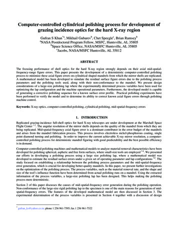
1.8RC lap1.6Gugolz 73 pitch tool1.4 4 99(x- 0 0}3)YI 0.60.4y - 0.72(x - e 3. Measured smoothing factor as a function of the initial PV irregularity for classical tool withGugolz 73 pitch and for the RC lap with LP66 polishing pads.5 Note that this work calculates thesmoothing factor with ε defined as PV irregularity for sinusoidal ripples a fixed frequency.The results of the controlled smoothing experiments are striking. For both types of tools, the smoothing factor has alinear variation with ε0 the initial surface irregularity and both go to zero at a threshold value, below which no smoothingoccurs. As shown in Figure 3, the value of the slope and threshold vary for different polishing processes. Fitting thedata to two parameters, the smoothing factor can be approximated asSF k ( ε ini ε 0 )Eq. 2This work has been extended to high spatial frequencies, evaluating the evolution of the power spectral density (PSD)for various lap types. Figure 4. shows an evolution of the high frequency PSD as a surface is polished usingconventional pitch #64 with Opaline polishing compound. 610 10'- CP #64, .3 PSI, Opaline 1 hou- CP 464, .3 PSI, Opaline 2 hou104 -CP 464, .3 PSI, Opaline 3 hoursCP #64, .3 PSI, Opaline 5 hoursCP #64, .3 PSI, Opaline 8 hours10'10 1010210'spatial frequency (cycles /mm)Figure 4. The surface high frequency irregularity relies entirely on natural smoothing. This figureshows the evolution of the high frequency PSD as the surface is polished using Opaline polishingcompound with a lap made of #64 pitch.6Proc. of SPIE Vol. 9151 91512R-3Downloaded From: http://proceedings.spiedigitallibrary.org/ on 01/21/2015 Terms of Use: http://spiedl.org/terms
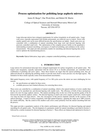
The smoothing factor as defined above works well for the case where well-defined sinusoidal irregularities are improvedby natural smoothing under controlled tests. This allows the smoothing effect of polishing tools to be engineered andmeasured explicitly. 7 But surfaces being fabricated are much more complex. Rather than a single frequency, a fullspectrum of irregularities is always present. In addition to the natural smoothing that improves the surface, someartifacts are frequently created by imperfect tool behavior. Also the measurements are never perfect, and the ability toaccurately assess smoothing relies on subtracting data sets, which inherently amplifies any noise. These effects areaccommodated for real polishing runs using a correlation based smoothing model where the smoothing factor includesonly changes in the surface that are correlated with the initial surface irregularities. 8 The smoothing factor applies forthis case, but the definition of εini and ε’ are changed to the root mean squared irregularity with period smaller than thetool.The correlated smoothing was quantified for two different types of tools running on 8.4-m mirrors. The same linearbehavior of the smoothing factor as described by Eq. 2 was maintained for different size and type of laps, faced withpitch or polishing pads. Figure 5 shows the 80-cm diameter (contact area) stressed lap shown polishing the LSSTtertiary mirror and a 25-cm Rigid Conformal (RC) tool polishing one of the GMT primary mirror segments.Figure 5. Large mirrors are polished with a variety of tools including the stressed lap shown polishing the LSST tertiary mirror on theleft and a rigid conformal tool working one of the GMT segments shown on the right.An example of the smoothing performance of the laps is provided for the case of the LSST tertiary mirror, polished byboth 80-cm stressed lap and 35-cm RC tools, both faced with LP66 polishing pads. The smoothing factor follows thesame linear trend, and is shown fit to this data in Figure 6.0.015Stressed lap with LP -66 on pitch-0- RC Lap with LP -660.012514.ó0.01--t; 0.0075SF 0.73(RMSini- 0.0034)s0.005SF 0.61(RMS .-0.0044 igure 6. Smoothing Factor from polishing runs on the LSST tertiary mirror for two types of laps.8Proc. of SPIE Vol. 9151 91512R-4Downloaded From: http://proceedings.spiedigitallibrary.org/ on 01/21/2015 Terms of Use: http://spiedl.org/terms
The smoothing factor provides useful information for a single polishing run. But this provides only a snapshot of thesurface improvement for this particular state. It is also useful to integrate the smoothing to evaluate the full evolution ofthe surface due to smoothing. It has been shown that the surface irregularity falls off as an exponential decay. 9 Weprovide an explicit derivation of this by combining Eq 1 and Eq. 2. and rewriting as a differential equation in Eq. 3where ε represents the RMS surface irregularity as a continuous function of DC removal z and ε0 is the threshold RMSirregularity, below which there appears no smoothing.ε ini ε ' zSF k ( ε ini ε 0 ) for a single polishing run dε ( z) d (ε ( z) ε 0 ) k ( ε ( z ) ε 0 )dzdzThe solution to Eq. 3 is simply an exponential, shown in Eq. 4. We define constant z0 ε ( z ) ε 0 ( ε ini ε 0 ) e zEq. 31and substitutekEq. 4z0Applying Eq. 4 to the data shown in Figure 6 is straightforward. Using data from the stressed lap, k 0.73 and ε0 is0.0034 µm. So z0 is 1.37 µm, which means that each time 1.37 µm is polished off of the surface, the irregularitybecomes 63% closer to the asymptotic value of ε0.surface irregularity (µm rms)0.160.14RC Lap0.12Stressed Lap0.10.080.060.040.020012345Total removal in microns678Figure 7. Exponential decay of the surface irregularity for a surface that starts with 0.14 µm rms, forpolishing with the RC lap and the stressed lap with smoothing factors shown in Figure 6.The optimization of the smoothing effect involves several parameters. The lap type, polishing compound, and stroke canbe chosen to provide the maximum smoothing effect.7,10 For a given process, the smoothing simply requires amplematerial removal. The total removal can be written using Preston’s equation as a function of the polishing time t as z (t )AlapAmirrorK P V twhereProc. of SPIE Vol. 9151 91512R-5Downloaded From: http://proceedings.spiedigitallibrary.org/ on 01/21/2015 Terms of Use: http://spiedl.org/termsEq. 5
Alap and Amirror are the respective areas of the polishing lap and the mirror being workedP is the lap pressureV is the mean velocity of the lap over the mirror surfaceK is Preston’s constant, 12 µm/hr / psi / (m/s) for cerium oxide polishing of borosilicate glassFor polishing of glass mirrors, we take the example of circular tools with the following: an orbital stroke with offset a of ¼ of the tool diameter DLAP, polishing pressure P, typically 0.3 psi stroking speed, Ω typically 30 – 90 rpm Instantaneous lap velocity V 2πa Ω/60 (a in meters, Ω in RPM, V in m/s)The removal as a function of time is simply z (t )2Dlap2mirrorD3Dlap ΩDlap) t 0.026 2KP(2πKPΩt4 60DmirrorEq. 6whereDlap and Dmirror are the respective diameters of the polishing lap and the mirror in meterst is the machine time in hoursz(t) is the removal in micronsSince removal and time are proportional, we can simply evaluate the time constant for the exponential surfaceimprovement as τ whereτ 382Dmirrorz03DlapKPΩEq. 7Figure 8 illustrates the case of a 1-m mirror polished with a 0.6-m lap at 10 rpm, we can expect a 1/e time constant forthe smoothing of the surface irregularity of 6.7 hours. It will take 2.3 times this, or 15 machine hours to improve thesurface irregularity above the threshold by a factor of 10.0.50initialSurface profile (µm)-0.5-14 hours-1.58 hours-2-2.512 hours-316 hours-3.5Figure 8. Evolution of a surface that starts with 0.14 µm rms, and is polished with a stressed lap withsmoothing factor shown in Figure 6, with z0 of 1.37 µm and ε0 of 0.0034 µm.Proc. of SPIE Vol. 9151 91512R-6Downloaded From: http://proceedings.spiedigitallibrary.org/ on 01/21/2015 Terms of Use: http://spiedl.org/terms
3. DIRECTED FIGURINGOptical surfaces are finished using a combination of smoothing described above and directed figuring, in which theprocess is adjusted to achieve removal variations across the work piece. The most common method uses dwell time –the tool spends more time over regions that require more removal. The tool influence function is calibrated, and thedwell time is optimized for each position on the mirror. 11 This process is fundamentally different than natural smoothingbecause it relies on the accuracy of the surface measurements and on the ability of the polishing mechanism to provideaccurate and stable removal. Directed removal is quite effective when the polishing machine spends more time on highregions and avoids low regions, as correctly provided by the measurements. However, directed figuring can degrade thesurface if there are errors in the data (either magnitude of irregularity or the mapping) or if the removal is not predictable(either in the wear rate, profile, or position.)The efficiency of the directed figuring can be quantified in a similar manner as the natural smoothing. However, wemust accommodate two principal differences. The smoothing appears to be fairly constant for irregularities withdifferent periods as long as they are small compared to the lap size. Larger periods are not affected by smoothing. Theconvergence of directed figuring is excellent for spatial periods that are large compared to the lap. The effect on smallerperiods is nonlinear. The directed figuring may improve the frequency being addressed, but will create higher frequencyerrors that are referred to as “tool marks.”We perform direct evaluation for circular tools that are driven in a circular orbit. Such a tool creates removal accordingto the Tool Influence Function (TIF) shown in Figure 9. We evaluate the ability to correct a range of frequencies bydirect simulation using a surface with 200 mm period, 0.4 µm PV, 0.14 µm rms sinusoidal ripples, as shown in Figure10. Different sized tools are used for simulations that each target the sinusoidal error. The polishing time and theresidual after correction are used to determine normalized performance parameters.Static TIF (3D View)Static TIF (Top View)OLI.-250-50Y (mm)5000-50X0-60(rnm)50X (mm)Static TIF Profile in YStatic TIF Profile in X0o0J-O3E-1.5-50500-50X (mm)060Y (mm)Figure 9. Example of a Tool Influence Function (TIF) for a 120 mm diameter tool stroked with anorbital radius of 30 mm.Proc. of SPIE Vol. 9151 91512R-7Downloaded From: http://proceedings.spiedigitallibrary.org/ on 01/21/2015 Terms of Use: http://spiedl.org/terms
Imported Map (3D View)Imported Map (Top View)-500ÉV 0.4E0E}500500-5000X (mm)Imported Map Profile in XImported Map Profile in Y0.41.5ÊÊ . 3 0.30.2 0.10LIIII-500.5000 1050-0.5G -1-500X (mm)0Y500(mm)Figure 10. A 1-m surface with 0.14 µm rms ripples at 200 mm periods was used to determineperformance of optimized polishing with different tool sizes.The dwell time for each run was fully optimized to minimize the rms residual, after the run is finished. An example isshown in Figure 11, showing a simulation of a 120 mm tool, running with 30 mm orbital stroke radius at 100 rpm and0.3 psi. The operation takes 14.6 hours to minimize the rms, leaving a residual of 0.008 µm rms.0.45Absolute Surface Profile (μm)0.4initial0.350.33.65 hours0.257.60 hours0.20.1510.9 hours0.10.0514.6 hours0-0.05Figure 11. Evolution of a surface that starts with 0.14 µm rms, and is polished with an optimal strokewith a 180 mm diameter TIF.Proc. of SPIE Vol. 9151 91512R-8Downloaded From: http://proceedings.spiedigitallibrary.org/ on 01/21/2015 Terms of Use: http://spiedl.org/terms
0.163500.14Final Surface RMS (μm)Run Time 0100200300TIF Diameter (mm)04000100200300TIF Diameter (mm)400Figure 12. Optimization simulation runs were performed to correct sinusoidal irregularity with 0.4 µm PV(0.14 µm rms) and 200 mm period for a 1-m optic. The Tool Influence Function diameter was varied fromone run to the next. The total polishing time and the residual after optimization are shown here.These data are normalized into two functions: Efficiency, defined as the improvement in the surface per micron of mean removal, units are µm rms/µm. Normalized Residual, defined as the rms residual created per rms corrected, units are µm rms/µm rmsBoth the efficiency and the normalized residual show a transition zone between tools being large compared to the periodand tools that are small. Such data is well fit using a classic sigmoid or S-curve function, which is generally writtenusing three parameters, A, D½ , and w.AS ( D) 1 e Eq. 8( D D1/2 )w0.400.35Simulated performance0.30Sigmoid FitNormalized Residual (µm rms residual/ µmrms correction)Efficiency (µm rms correction/µm removal)The data from Figure 12 is normalized and fit to the sigmoid function, as shown in Figure 13. The values from the fitare provided in Table 1. Note that these are normalized, so they can be easily scaled for any size tool or any 1.21.4Normalized spatial frequency (cycles/tool diameter)1.61.2Simulated performance1Sigmoid Fit0.80.60.40.2000.20.40.60.811.21.4Normalized spatial frequency (cycles/tool diameter)Figure 13. Normalized parameters taken from the simulations for orbital polishing of sinusoidal surfaceirregularity as a function of the spatial frequency. A 3-parameter sigmoid fit is used to describe the data.Proc. of SPIE Vol. 9151 91512R-9Downloaded From: http://proceedings.spiedigitallibrary.org/ on 01/21/2015 Terms of Use: http://spiedl.org/terms1.6
Table 1. Sigmoid fit parameters from the data in Figure 13.EfficiencyNormalized ResidualA0.37 µm rms/µm0.98 µm rms/µm rmsD½0.93 cycles/tool diameter1.00 cycles/tool diameterw-0.145 cycles/tool diameter0.126 cycles/tool diameter4. PROCESS OPTIMIZATIONThe parametric relations for smoothing and for directed removal allow quantitative predictions of performance withoutperforming simulations. Such predictions lend themselves to parametric process optimization, where parameters thatdescribe the manufacturing can be adjusted and optimize to produce higher performance surfaces or to increaseefficiency. As an example for this paper, we choose to evaluate the polishing of a 1-m diameter surface. We evaluatethe improvement of surface error with 200 mm period.We already showed the surface improvement due to natural smoothing with a 600 mm lap. We compare this with theperformance of a small tool using directed figuring. The orbital speed is 100 rpm, the pressure is 0.3 psi, and the Prestonconstant is 12 µm/(m/s)/psi/hr. Figure 14 clearly shows a few points: Smoothing is superior to directed figuring for the case where the smoothing lap is greater than several periodsacross and irregularities are large. Directed figuring with tools that are greater than 70% of the period shows good efficiency, but the residualcreated is too large. The data should be filtered before optimization to avoid such problems. The tools smaller than 70% of the period create very little residual, but are extremely slow.0.1610.140.80.71Lap diam/period0.90.12Lap diameter/cycle0.80.60.1Smoothing tool0.140.90.120.5Residual (µm rms)Surface irregularity (µm rms)0.16Smoothing 0246810121416182002468101214161820Time in hoursTime in hoursFigure 14. Surface evolution for directed figuring with laps that vary from 1 x the spatial period of theripples to ½ times this period. As the sinusoidal irregularity improves for the case of directed figure, thesmaller scale residual grows. As the smoothing tool operates, the residual amount of the originalirregularity decreases exponentially.It is instructive to evaluate the rate of change of the surface irregularity, which is readily provided using the parametricmodels. Figure 15 shows the rate of improvement due to natural smoothing and Figure 16 shows the rates for directedfiguring (surface correction and creation of residual) as functions of the tool size.Proc. of SPIE Vol. 9151 91512R-10Downloaded From: http://proceedings.spiedigitallibrary.org/ on 01/21/2015 Terms of Use: http://spiedl.org/terms
smoothing rate (µm 40Polishing time in hours00.007-0.0020.006Residual rate (µm rms/hr)Correction rate (µm rms/hr)Figure 15. Rate of change for surface irregularity due to natural smoothing with a 60 cm ormalized frequency (cycles/tool diameter)0.400.600.801.001.201.40Normalized frequency (cycles/tool diameter)Figure 16. Rate of change for surfaces due to directed figuring with different size tools as described above.Improved efficiency and final surface quality can be achieved using a combination of two tools:1.Use a large smoothing tool first. Continue until the rate of improvement of the smoothing is less than that fordirected figuring2.Switch to small tool directed figuring. Evaluate time to complete and the residual tool marks created from thisIf necessary, even smaller tools could be used to correct the tool marks or other errors introduced into the surface, 12 orspecialized tools can be run on the edges. 13 We evaluate an optimized two-step process for various sizes of orbital tools,but the transition point for each is optimized to occur when the correction rate matches the smoothing rate. A set ofcases with different tools is shown in Figures 17 and 18. These figures illustrate an important tradeoff betweenefficiency and final quality. Compare the performance of the tool that is 0.5 times the period with the largest oneconsidered here, with diameter 0.8 times the period. The smaller tool performs better, achieving surface quality below0.001 µm rms in 20 hours. But most surfaces do not require such quality. The larger tool can achieve 0.012 µm rms inonly 11 hours. The smaller tool requires 16 hours to achieve the same results.Proc. of SPIE Vol. 9151 91512R-11Downloaded From: http://proceedings.spiedigitallibrary.org/ on 01/21/2015 Terms of Use: http://spiedl.org/terms
0.16Surface irregularity (µm rms)0.14Smoothing tool0.80.120.70.1Lap sizeper period0.60.50.080.060.040.0200510Time in hours1520Figure 17. Evolution of the surface figure for an optimized combination of a 60 cm smoothing toolfollowed with small tool directed figuring. The transition point between the two operations is optimallychosen to occur when the directed removal rate just exceeds that of passive smoothing.Surface irregularity (µm rms)1Smoothing tool0.8Lap size0.7per period0.60.50.10.010.0010510Time in hours15Figure 18. Same data as shown in Figure 17, shown here on a log scale.Proc. of SPIE Vol. 9151 91512R-12Downloaded From: http://proceedings.spiedigitallibrary.org/ on 01/21/2015 Terms of Use: http://spiedl.org/terms20
5. CONCLUSIONWe provide parametric relations that allow quantitative estimate of the performance of the polishing process in terms ofthe natural smoothing of features smaller than the lap and directed figuring for features larger than the lap. The initialevaluation of the simple case of a single sinusoidal surface error shows the value of these models. The parametricrelations can be used to optimize the choice of the polishing tool for directed figuring to either achieve the fastest or thehighest quality result. A more general solution can be built into the SAGUARO processing platform 14 thataccommodates a complete power spectrum. Also, these models can be extended to loose abrasive grinding or shearmode grinding. 15We note that this analysis simplifies a complex interaction between the surface measurement uncertainty and the choiceof parameters. For example, the choice of using the smallest tool allows correction with the least residual, but this ismost sensitive to errors in the measurements that are used to optimize the polishing run and to instability or inaccuracyof the polishing tool. A variety of surface measurement techniques are used to provide a full range of spatial frequencyinformation. 16 If the confidence in metrology and polishing controls could also be quantified, then this informationcould also be applied to optimize the full process.REFERENCES1) M. Tuell, J. H. Burge, and B. Anderson, “Aspheric optics: smoothing the ripples with semi-flexible tools.” Optical Engineering41(7) pp. 1473-1474 (2002).2) D. W. Kim and J. H. Burge, “Rigid conformal polishing tool using non-linear visco-elastic effect,” Opt. Express 18, 2242-2257(2010).3) H. M. Martin, R. G. Allen, J. H. Burge, B. Cuerden, D. W. Kim, J. S. Kingsley, K. Law, R. Lutz, P. A. Strittmatter, P. Su, M. T.Tuell, S. Warner, S. C. West, P. Zhou, “Production of 8.4 m segments for the Giant Magellan Telescope,” Proc. SPIE 8450(2012).4) M. T. Tuell, H. M. Martin, J. H. Burge, D. A. Ketelsen, K. Law, W. J. Gressler, C. Zhao, “Fabrication of the LSST monolithicprimary-tertiary mirror,” Proc. SPIE 8450 (2012).5) D. W. Kim, W. H. Park, H. K. An, and J. H. Burge, “Parametric smoothing model for visco-elastic polishing tools,” Opt. Express18, 22515-22526 (2010).6) J. G. Del Hoyo, DW. Kim, J. H. Burge, “Super-smooth optical fabrication controlling high-spatial frequency surface irregularity,”Proc. SPIE 8838, 88380T (2013).7) X. Nie, S. Li, F. Shi, and H. Hu, "Generalized numerical pressure distribution model for smoothing polishing of irregularmidspatial frequency errors," Appl. Opt. 53, 1020-1027 (2014).8) Y. Shu, D. Kim, H. Martin, and J. H. Burge, “Correlation-based smoothing model for optical polishing,” Opt. Express 21, 2877128782 (2013).9) Y. Shu, X. Nie, F. Shi, and S. Li, “Smoothing evolution model for computer controlled optical surfacing,” J. Opt. Technol. 81 (3),(2014).10) Y. Shu, X. Nie, F. Shi, S. Li, “Compare study between smoothing efficiencies of epicyclic motion and orbital motion,” Optik(2014)11) D. W. Kim, H. M. Martin, J. H. Burge, “Calibration and optimization of computer-controlled optical surfacing for large optics,”Proc. SPIE 8126 (2011).12) D. W. Kim, S. W. Kim, and J. H. Burge, “Non-sequential optimization technique for a computer controlled optical surfacingprocess using multiple tool influence functions,” Opt. Express 17, 21850-21866 (200913) D. W. Kim, W. H. Park, S.-W. Kim, and J. H. Burge, “Parametric modeling of edge effects for polishing tool influence functions,”Opt. Express 17, 5656-5665 (2009).14) D. W. Kim, B. J. Lewis, J. H. Burge, “Open-source data analysis and visualization software platform: SAGUARO,” Proc. SPIE8126 (2011).15) J. B. Johnson, D. W. Kim, R. E. Parks, and J. H. Burge, “New approach for pre-polish grinding with low subsurface damage,”Proc. SPIE 8126 (2011).16) M. J. Valente, B. J. Lewis, N. Melena, M. A. Smith, J. H. Burge, “Advanced surface metrology for meter-class optics,” Proc. SPIE8838, 88380F (2013).Proc. of SPIE Vol. 9151 91512R-13Downloaded From: http://proceedings.spiedigitallibrary.org/ on 01/21/2015 Terms of Use: http://spiedl.org/terms
pitch or polishing pads. Figure 5 shows the 80-cm diameter (contact area) stressed lap shown polishing the LSST tertiary mirror and a 25-cm Rigid Conformal (RC) tool polishing one of the GMT primary mirror segments. Figure 5. Large mirrors are polished with a variety of tools including the stressed lap shown polishing the LSST tertiary mirror .