Transcription
Wesley W. ChuT. Y. LinEditorsFoundations and Advancesin Data MiningSpringer-Verlag
Professor Dr. Wesley W. ChuComputer Science DepartmentUniversity of California, Los AngelesCalifornia, 90095wwc@cs.ucla.eduProfessor Dr. Tsau Young LinDepartment of Computer Science,San Jose State UniversitySan Jose, CA 95192tylin@cs.sjsu.edu
PrefaceWith the growing use of information technology and the recent advances in websystems, the amount of data available to users has increased exponentially. Thus, there isa critical need to understand the content of the data. As a result, data-mining has becomea popular research topic in recent years for the treatment of the “data rich and informationpoor” syndrome. Currently, application oriented engineers are only concerned with theirimmediate problems, which results in an ad hoc method of problem solving. Researchers,on the other hand, lack an understanding of the practical issues of data-mining for realworld problems and often concentrate on issues (e.g. incremental performanceimprovements) that are of no significance to the practitionersIn this volume, we hope to remedy these problems by (1) presenting a theoreticalfoundation of data-mining, and (2) providing important new directions for data-miningresearch. We have invited a set of well respected data mining theoreticians to presenttheir views on the fundamental science of data mining. We have also called onresearchers with practical data mining experiences to present new important data-miningtopics.This book is organized into two parts. The first part consists of four chapterspresenting the foundations of data mining, which describe the theoretical point of viewand the capabilities and limits of current available mining techniques. The second partconsists of seven chapters which discuss the new data mining topics.The first part of the book includes four chapters. The first chapter, authored by T.Poggio and S. Smale, is entitled “The Mathematics of Learning: Dealing with Data.”The authors present the mathematical formula of learning theory. In particular, theypresent an algorithm for supervised learning by training sets and show that the algorithmperforms well in a number of applications involving regression as well as binaryclassification. The second chapter, by H. Tsukimoto, is entitled “Logical RegressionAnalysis: From Mathematical Formulas to Linguistic Rules.” He presents a solution forsolving the accurate prediction and comprehensive rules in supervised learning. Theauthor has developed a data mining technique called Logical Regression Analysis whichconsists of regression analysis, and the Approximation Method, that can providecomprehensive rules and also accurate prediction. The paper also shows how to applythe techniques for mining images. The third chapter, by T.Y. Lin, is entitled “ AFeature/Attribute Theory for Association Mining and Constructing the Complete FeatureSet” The author points out the importance of selecting correct attributes in data miningand develops a theory of features for association mining (AM). Based on theisomorphism theorem in AM, he concludes that it is sufficient to perform AM incanonical models, and constructs the complete feature set for every canonical model.Using the isomorphism theorem, the complete feature set can be derived for each relation.Though the number of possible features is enormous, it can be shown that the highfrequency patterns features can be derived within polynomial time. The fourth chapter isentitled “A new theoretical framework for K-means-type clustering,” and is authored by J.
VIPrefacePeng and Y. Xia. The authors present generalized K-means type clustering method as the0-1 semi-definite programming (SDP). The classical K-means algorithm, minimal sumof squares (MSSC), can be interpreted as a special heuristic. Moreover, the 0-1 SDPmodel can be further approximated by the relaxed and polynomially solvable linear andsemi-definite programming. The 0-1 SDP model can be applied to MSCC and to otherscenarios of clustering as well.The second part of the book, from Chapters 5 to 11, present seven topics coveringrecent advances in data mining. Chapter 5, entitled “Clustering via Decision TreeConstruction,” is authored by B. Liu, Y. Xia, and P. Yu. They propose a novel clusteringtechnique based on supervised learning called decision tree construction. The key idea isto use a decision tree to partition the data space into cluster (or dense) regions and empty(or sparse) regions (which produce outliers and anomalies). This technique is able to find“natural” clusters in large high dimensional spaces efficiently. Experimental data showsthat this technique is effective and scales well for large high dimensional datasets.Chapter 6, “Incremental Mining on Association Rules,” is written by Wei-Guang Tengand Ming-Syan Chen. Due to the increasing use of the record-based databases where datais being constantly added, incremental mining is needed to keep the knowledge current.The authors propose incremental mining techniques to update the data mining onassociation rules. Chapter 7, is entitled “Mining Association Rules from Tabular DataGuided by Maximal Frequent Itemsets” and authored by Q. Zou, Y. Chen, W. Chu, andX. Lu. Since many scientific applications are in tabular format, the authors propose touse the maximum frequency itemset (MFI) as a road map to guide us towards generatingassociation rules from tabular dataset. They propose to use information from previoussearches to generate MFI and the experimental results show that such an approach togenerating MFI yields significant improvements over conventional methods. Further,using tabular format rather than transaction data set to derive MFI can reduce the searchspace and the time needed for support-counting. The authors use spreadsheet to presentrules and use spreadsheet operations to sort and select rules, which is a very convenientway to query and organize rules in a hierarchical fashion. An example was also given toillustrate the process of generating association rules from the tabular dataset using pastmedical surgery data to aid surgeons in their decision making. Chapter 8, entitled“Sequential Pattern Mining by Pattern-Growth: Principles and Extensions,” presents thesequential pattern growth method and studies the principles and extensions of the methodsuch as (1) mining constraint-based sequential patterns, (2) mining multi-level, multidimensional sequential patters, and (3) mining top-k closed sequential patterns. They alsodiscuss the applications in bio-sequence pattern analysis and clustering sequences.Chapter 9, entitled “Web Page Classification,” is written by B. Choi and Z. Yao. Itdescribes systems that automatically classify web pages into meaningful subject-basedand genre-based categories. The authors describe tools for building automatic web pageclassification systems, which are essential for web mining and constructing semantic web.Chapter 10 is entitled “Web Mining – Concepts, Applications, and Research Directions,”and was written by Jaideep Srivastava, Prasanna Desikan, and Vipin Kumar. The authorspresent the application of data mining techniques to extract knowledge from web content,structure, and usage. An overview of accomplishments in technology and applications inweb mining is also included. Chapter 11, by Chris Clifton, Murat Kantarcioglu, and
PrefaceVIIJaideep Vaidya is entitled, “Privacy-Preserving Data Mining.” The goal of privacypreserving data mining is to develop data mining models that do not increase the risk ofmisuse of the data used to generate those models. The author presents two classes ofprivacy-preserving data-mining. The first is based on adding noise to the data beforeproviding it to the data miner. Since real data values are not revealed, individual privacyis preserved. The second class is derived from the cryptographic community. The datasources collaborate to obtain data mining results without revealing anything except thoseresults.Finally, we would like to thank the authors for contributing their work in thevolume and the reviewers for commenting on the readability and accuracy of the work.We hope the theories presented in this volume will give data mining practitioners ascientific perspective in data mining and thus provide more insight into their problems.We also hope that the new data mining topics will stimulate further research in theseimportant directions.Wesley W. Chu and T. Y. Lin
Table of ContentsPart IFoundations of Data Mining ---------1The Mathematics of -----------------Tomaso Poggio, Steve Smale3Logical Regression Analysis: From Mathematical Formulas to Linguistic RulesHiroshi Tsukimoto19A Feature/Attribute Theory for Association Mining and Constructing theComplete Feature ----------------------Tsau-Young LinA New Theoretical Framework for K-means-type Clustering----------------------Jiming Peng, Yu XiaPart IIRecent Advances in Data Mining ---617795Clustering via Decision Tree ------Bing Liu, Yiyuan Xia, Philip S. Yu97Incremental Mining on Association Wei-Guang Teng, Ming-Syan Chen123Mining Association Rules from Tabular Data Guided by Maximal -Qinghua Zou, Yu Chen, Wesley W. Chu, Xinchun Lu161Sequential Pattern Mining by Pattern-Growth: Principles and Extensions-------Jiawei Han, Jian Pei, Xifeng Yan181Web Page -----------------------------Ben Choi, Zhongmei Yao217
XTable of ContentsWeb Mining – Concepts, Applications, and Research Directions-----------------Jaideep Srivastava, Prasanna Desikan, Vipin Kumar279Privacy-Preserving Data ----------Chris Clifton, Murat Kantarcioglu, Jaideep Vaidya313
Part IFoundations of Data Mining
The Mathematics of Learning: Dealing with Data?Tomaso Poggio1 and Steve Smale21CBCL, McGovern Institute, Artificial Intelligence Lab, BCS, MIT, tp@ai.mit.eduToyota Technological Institute at Chicago and Professor in the Graduate School,University of California, Berkeley, smale@math.berkeley.edu2Summary. Learning is key to developing systems tailored to a broad range of data analysisand information extraction tasks. We outline the mathematical foundations of learning theoryand describe a key algorithm of it.1 IntroductionThe problem of understanding intelligence is said to be the greatest problem in science today and “the” problem for this century - as deciphering thegenetic code was for the second half of the last one. Arguably, the problemof learning represents a gateway to understanding intelligence in brains andmachines, to discovering how the human brain works and to making intelligent machines that learn from experience and improve their competences aschildren do. In engineering, learning techniques would make it possible todevelop software that can be quickly customized to deal with the increasingamount of information and the flood of data around us. Examples abound.During the last decades, experiments in particle physics have produced avery large amount of data. Genome sequencing is doing the same in biology. The Internet is a vast repository of disparate information which changesrapidly and grows at an exponential rate: it is now significantly more than100 Terabytes, while the Library of Congress is about 20 Terabytes. We believe that a set of techniques, based on a new area of science and engineeringbecoming known as “supervised learning” – will become a key technologyto extract information from the ocean of bits around us and make sense ofit. Supervised learning, or learning-from-examples, refers to systems that aretrained, instead of programmed, with a set of examples, that is a set of inputoutput pairs. Systems that could learn from example to perform a specifictask would have many applications. A bank may use a program to screenloan applications and approve the “good” ones. Such a system would be?Reprinted by permission from Notices of the AMS, 50(5), 2003, pp.537–544
4Tomaso Poggio and Steve Smaletrained with a set of data from previous loan applications and the experiencewith their defaults. In this example, a loan application is a point in a multidimensional space of variables characterizing its properties; its associatedoutput is a binary “good” or “bad” label. In another example, a car manufacturer may want to have in its models, a system to detect pedestrians thatmay be about to cross the road to alert the driver of a possible danger whiledriving in downtown traffic. Such a system could be trained with positiveand negative examples: images of pedestrians and images without people.In fact, software trained in this way with thousands of images has been recently tested in an experimental car of Daimler. It runs on a PC in the trunkand looks at the road in front of the car through a digital camera [36, 26, 43].Algorithms have been developed that can produce a diagnosis of the type ofcancer from a set of measurements of the expression level of many thousandshuman genes in a biopsy of the tumor measured with a cDNA microarraycontaining probes for a number of genes [46]. Again, the software learns theclassification rule from a set of examples, that is from examples of expression patterns in a number of patients with known diagnoses. The challenge,in this case, is the high dimensionality of the input space – in the order of20, 000 genes – and the small number of examples available for training –around 50. In the future, similar learning techniques may be capable of somelearning of a language and, in particular, to translate information from onelanguage to another. What we assume in the above examples is a machinethat is trained, instead of programmed, to perform a task, given data of theform (xi , yi )mi 1 . Training means synthesizing a function that best representsthe relation between the inputs xi and the corresponding outputs yi . The central question of learning theory is how well this function generalizes, that ishow well it estimates the outputs for previously unseen inputs.As we will see later more formally, learning techniques are similar to fitting a multivariate function to a certain number of measurement data. Thekey point, as we just mentioned, is that the fitting should be predictive, in thesame way that fitting experimental data (see figure 1) from an experiment inphysics can in principle uncover the underlying physical law, which is thenused in a predictive way. In this sense, learning is also a principled methodfor distilling predictive and therefore scientific “theories” from the data. Webegin by presenting a simple “regularization” algorithm which is importantin learning theory and its applications. We then outline briefly some of itsapplications and its performance. Next we provide a compact derivation ofit. We then provide general theoretical foundations of learning theory. In particular, we outline the key ideas of decomposing the generalization error ofa solution of the learning problem into a sample and an approximation error component. Thus both probability theory and approximation theory playkey roles in learning theory. We apply the two theoretical bounds to the algorithm and describe for it the tradeoff – which is key in learning theory andits applications – between number of examples and complexity of the hypothesis
The Mathematics of Learning: Dealing with Data5Fig. 1. How can we learn a function which is capable of generalization – among the manyfunctions which fit the examples equally well (here m 7)?space. We conclude with several remarks, both with an eye to history and toopen problems for the future.2 A key algorithm2.1 The algorithmHow can we fit the “training” set of data Sm (xi , yi )mi 1 with a functionf : X Y – with X a closed subset of IRn and Y IR – that generalizes, egis predictive? Here is an algorithm which does just that and which is almostmagical for its simplicity and effectiveness:1. Start with data (xi , yi )mi 102. Choose a symmetric, positive definite function Kx (xP) K(x, x0 ), continnuous on X X. A kernel K(t, s) is positive definite ifi,j 1 ci cj K(ti , tj ) 0 for any n IN and choice of t1 , ., tn X and c1 , ., cn IR. An example of such a Mercer kernel is the GaussianK(x, x0 ) e restricted to X X.3. Set f : X Y tof (x) mXi 1kx x0 k22σ 2.(1)ci Kxi (x).(2)
6Tomaso Poggio and Steve Smalewhere c (c1 , ., cm ) and(mγI K)c y(3)where I is the identity matrix, K is the square positive definite matrixwith elements Ki,j K(xi , xj ) and y is the vector with coordinates yi .The parameter γ is a positive, real number.The linear system of equations 3 in m variables is well-posed since K is positive and (mγI K) is strictly positive. The condition number is good if mγis large. This type of equations has been studied since Gauss and the algorithms for solving it efficiently represent one the most developed areas in numerical and computational analysis. What does Equation 2 say? In the caseof Gaussian kernel, the equation approximates the unknown function by aweighted superposition of Gaussian “blobs” , each centered at the locationxi of one of the m examples. The weight ci of each Gaussian is such to minimize a regularized empirical error, that is the error on the training set. Theσ of the Gaussian (together with γ, see later) controls the degree of smoothing, of noise tolerance and of generalization. Notice that for Gaussians withσ 0 the representation of Equation 2 effectively becomes a “look-up” tablethat cannot generalize (it provides the correct y yi only when x xi andotherwise outputs 0).2.2 Performance and examplesThe algorithm performs well in a number of applications involving regression as well as binary classification. In the latter case the yi of the trainingset (xi , yi )mi 1 take the values { 1, 1}; the predicted label is then { 1, 1},depending on the sign of the function f of Equation 2. Regression applications are the oldest. Typically they involved fitting data in a small numberof dimensions [53, 44, 45]. More recently, they also included typical learningapplications, sometimes with a very high dimensionality. One example isthe use of algorithms in computer graphics for synthesizing new images andvideos [38, 5, 20]. The inverse problem of estimating facial expression andobject pose from an image is another successful application [25]. Still anothercase is the control of mechanical arms. There are also applications in finance,as, for instance, the estimation of the price of derivative securities, such asstock options. In this case, the algorithm replaces the classical Black-Scholesequation (derived from first principles) by learning the map from an inputspace (volatility, underlying stock price, time to expiration of the option etc.)to the output space (the price of the option) from historical data [27]. Binary classification applications abound. The algorithm was used to performbinary classification on a number of problems [7, 34]. It was also used to perform visual object recognition in a view-independent way and in particularface recognition and sex categorization from face images [39, 8]. Other applications span bioinformatics for classification of human cancer from microar-
The Mathematics of Learning: Dealing with Data7ray data, text summarization, sound classification3 Surprisingly, it has beenrealized quite recently that the same linear algorithm not only works wellbut is fully comparable in binary classification problems to the most popularclassifiers of today (that turn out to be of the same family, see later).2.3 DerivationThe algorithm described can be derived from Tikhonov regularization. Tofind the minimizer of the the error we may try to solve the problem – calledEmpirical Risk Minimization (ERM) – of finding the function in H whichminimizesm1 X(f (xi ) yi )2m i 1which is in general ill-posed, depending on the choice of the hypothesis spaceH. Following Tikhonov (see for instance [19]) we minimize, instead, overthe hypothesis space HK , for a fixed positive parameter γ, the regularizedfunctionalm1 X(yi f (xi ))2 γkf k2K ,(4)m i 1where kf k2K is the norm in HK – the Reproducing Kernel Hilbert Space(RKHS), defined by the kernel K. The last term in Equation 4 – called regularizer – forces, as we will see, smoothness and uniqueness of the solution.Let us first define the norm kf k2K . Consider the space of the linear span ofKxj . We use xj to emphasize that the elements of X used in this constructiondo not have anything to do in general with the training set (xi )mi 1 . Define aninner productinthisspacebysettinghK,Ki K(x,x)andextend linxxjjPrearly to j 1 aj Kxj . The completion of the space in the associated norm isthe RKHS, that is a Hilbert space HK with the norm kf k2K (see [10, 2]). Notethat hf, Kx i f (x) for f HK (just let f Kxj and extend linearly). Tominimize the functional in Equation 4 we take the functional derivative withrespect to f , apply it to an element f of the RKHS and set it equal to 0. Weobtainm1 X(yi f (xi ))f (xi ) γhf, f i 0.(5)m i 1Equation 5 must be valid for any f . In particular, setting f Kx givesf (x) mXci Kxi (x)(6)i 13The very closely related Support Vector Machine (SVM) classifier was used forthe same family of applications, and in particular for bioinformatics and for facerecognition and car and pedestrian detection [46, 25].
8Tomaso Poggio and Steve Smalewhereci yi f (xi )mγ(7)since hf, Kx i f (x). Equation 3 then follows, by substituting Equation6 into Equation 7. Notice also that essentially the same derivation for ageneric loss function V (y, f (x)), instead of (f (x) y)2 , yields the same Equation 6, but Equation 3 is now different and, in general, nonlinear, depending on the form of V . In particular, the popular Support Vector Machine(SVM) regression and SVM classification algorithms correspond to specialchoices of non-quadratic V , one to provide a ’robust” measure of error andthe other to approximate the ideal loss function corresponding to binary(miss)classification. In both cases, the solution is still of the same form ofEquation 6 for any choice of the kernel K. The coefficients ci are not givenanymore by Equations 7 but must be found solving a quadratic programming problem.3 TheoryWe give some further justification of the algorithm by sketching very brieflyits foundations in some basic ideas of learning theory. Here the data (xi , yi )mi 1is supposed random, so that there is an unknown probability measure ρ onthe product space X Y from which the data is drawn. This measure ρ defines a functionfρ : X Y(8)Rsatisfying fρ (x) ydρx , where ρx is the conditional measure on x Y .From this construction fρ can be said to be the true input-output functionreflecting the environment which produces the data. Thus a measurement ofthe error of f isZ(f fρ )2 dρX(9)Xwhere ρX is the measure on X induced by ρ (sometimes called the marginalmeasure). The goal of learning theory might be said to “find” f minimizingthis error. Now to search for such an f , it is important to have a space H– the hypothesis space – in which to work (“learning does not take place in avacuum”). Thus consider a convex space of continuous functions f : X Y ,(remember Y IR) which as a subset of C(X) is compact, and where C(X) isthe Banach space of continuous functions with f maxX f (x) . A basicexample isH IK (BR )(10)where IK : HK C(X) is the inclusion and BR is the ball ofR in HK .Pradiusm12Starting from the data (xi , yi )m zonemayminimize(f(xi ) yi )i 1i 1mover f H to obtain a unique hypothesis fz : X Y . This fz is called theempirical optimum and we may focus on the problem of estimating
The Mathematics of Learning: Dealing with DataZ(fz fρ )2 dρX9(11)XIt is useful towards this end to break the problem into steps by definingaR“true optimum” fH relative to H, by taking the minimum over H of X (f fρ )2 . Thus we may exhibitZZ2(fz fρ ) S(z, H) (fH fρ )2 S(z, H) A(H)(12)XXwhereZS(z, H) (fz fρ )2 XZ(fH fρ )2(13)XThe first term, (S) on the right in Equation 12 must be estimated in probability over z and the estimate is called the sample errror (sometime also theestimation error). It is naturally studied in the theory of probability and of empirical processes [16, 30, 31]. The second term (A) is dealt with via approximation theory (see [15] and [12, 14, 13, 32, 33]) and is called the approximationerror. The decomposition of Equation 12 is related, but not equivalent, to thewell known bias (A) and variance (S) decomposition in statistics.3.1 Sample ErrorFirst consider an estimate for the sample error, which will have the form:S(z, H) (14)with high confidence, this confidence depending on and on the sample sizem. Let us be more precise. Recall that the covering number or Cov#(H, η) isthe number of balls in H of radius η needed to cover H.Theorem 3.1 Suppose f (x) y M for all f H for almost all (x, y) X Y .ThenP robz (X Y )m {S(z, H) } 1 δm )e 288M 2 .where δ Cov#(H, 24MThe result is Theorem C of [10], but earlier versions (usually without atopology on H) have been proved by others, especially Vapnik, who formulated the notion of VC dimension to measure the complexity of the hypothesis space for the case of {0, 1} functions. In a typical situation of Theorem 3.1the hypothesis space H is taken to be as in Equation 10, where BR is the ballof radius R in a Reproducing Kernel Hilbert Space (RKHS) with a smoothK (or in a Sobolev space). In this context, R plays an analogous role to VCdimension[50]. Estimates for the covering numbers in these cases were provided by Cucker, Smale and Zhou [10, 54, 55]. The proof of Theorem 3.1 startsfrom Hoeffding inequality (which can be regarded as an exponential version
10Tomaso Poggio and Steve Smaleof Chebyshev’s inequality of probability theory). One applies this estimate tothe function X Y IR which takes (x, y) to (f (x) y)2 . Then extending theestimate to the set of f H introduces the covering number into the picture.With a little more work, theorem 3.1 is obtained.3.2 Approximation ErrorRThe approximation error X (fH fρ )2 may be studied as follows. SupposeB : L2 L2 is a compact, strictly positive (selfadjoint) operator. Then let Ebe the Hilbert space{g L2 , kB s gk }with inner product hg, hiE hB s g, B s hiL2 . Suppose moreover that E L2 factors as E C(X) L2 with the inclusion JE : E , C(X) welldefined and compact. Let H be JE (BR ) when BR is the ball of radius R in E.A theorem on the approximation error isTheorem 3.2 Let 0 r s and H be as above. Then2r2s1 s r rkfρ fH k ( )kB fρ k s rR2We now use k · k for the norm in the space of square integrable functions on1/2X, with measure ρX . For our main example of RKHS, take B LK , whereK is a Mercer kernel andZLK f (x) f (x0 )K(x, x0 )(15)Xand we have taken the square root of the operator LK . In this case E is HKas above. Details and proofs may be found in [10] and in [48].3.3 Sample and approximation error for the regularization algorithmThe previous discussion depends upon a compact hypothesis space H fromwhich the experimental optimum fz and the true optimum fH are taken. Inthe key algorithm of section 2 , the optimization is done over all f HKwith a regularized error function. The error analysis of sections 3.1 and 3.2must therefore be extended. Thus let fγ,z be the empirical optimum for theregularized problem as exhibited in Equation 4m1 X(yi f (xi ))2 γkf k2K .m i 1ThenZ(fγ,z fρ )2 S(γ) A(γ)(16)(17)
The Mathematics of Learning: Dealing with Data11where A(γ) (the approximation error in this context) is 1A(γ) γ 1/2 kLK 4 fρ k2(18)and the sample error isS(γ) 32M 2 (γ C)2 v (m, δ)γ2(19)where v (m, δ) is the unique solution ofm 34mv ln()v c1 0.4δ(20)Here C, c1 0 depend only on X and K. For the proof one reduces to thecase of compact H and applies theorems 3.1 and 3.2. Thus finding the optimalsolution is equivalent to finding the best tradeoff between A and S for a givenm. In our case, this bias-variance problem is to minimize S(γ) A(γ) overγ 0. There is a unique solution – a best γ – for the choice in Equation 4. Forthis result and its consequences see [11].4 RemarksThe tradeoff between sample complexity and hypothesis space complexity For agiven, fixed hypothesis space H only the sample error component of the errorof fz can be be controlled (in Equation 12 only S(z, H) depends on the data).In this view, convergence of S to zero as the number of data increases (theorem 3.1) is then the central problem in learning. Vapnik called consistency ofERM (eg convergence of the empirical error to the true error) the key problemin learning theory and in fact much modern work has focused on refiningthe necessary and sufficient conditions for consistency of ERM (the uniformGlivenko-Cantelli property of H, finite Vγ dimension for γ 0 etc., see [19]).More generally, however, there is a tradeoff between minimizing the sampleerror and minimizing the approximation error – what we referred to as thebias-variance problem. Increasing the number of data points m decreases thesample error. The effect of increasing the complexity of the hypothesis spaceis trickier. Usually the approximation error decreases but the sample errorincreases. This means that there is an optimal complexity of the hypothesisspace for a given number of training data. In the case of the regularizationalgorithm described in this paper this tradeoff corresponds to an optimumv
research. We have invited a set of well respected data mining theoreticians to present their views on the fundamental science of data mining. We have also called on researchers with practical data mining experiences to present new important data-mining topics. This book is organized