Transcription
Finding good nearly balanced cuts in power law graphsKevin Lang November 15, 2004AbstractIn power law graphs, cut quality varies inversely with cut balance. Using some million node social graphs as a testbed, we empirically investigate this property and its implications for graph partitioning. We use six algorithms, including Metis and MQI (state of the art methods for finding bisections and quotient cuts) and four relaxation/roundingmethods. We find that an SDP relaxation avoids the Spectral method’s tendency to break off tiny pieces of the graph.We also find that a flow-based rounding method works better than hyperplane rounding.1IntroductionWhile trying to partition some real-world power law graphs at Yahoo, we have encountered the problem that in thesegraphs cut quality varies inversely with cut balance. As illustrated by figure 2, in such graphs there are good cuts withbad balance and bad cuts with good balance, but there are no good cuts with good balance.1 Graph theorists havenoticed that power law graphs have this kind of structure [6], but the problem has not been discussed much in theempirical literature, which has mostly focused on finite element meshes and other classes of graphs where the bestquotient cut does not necessarily have bad balance.In this paper we investigate the behavior of six graph partitioning algorithms on power law graphs, specificallysocial graphs, with particular attention to the question of how one can find a cut that has good balance, and whosequotient cut score is as good as possible under that constraint. We find that an effective (but fairly expensive) approachconsists of first solving a semidefinite program (SDP) to obtain an embedding of the graph on a low-dimensionalhypersphere, and then using multiple tries of a randomized flow-based rounding method to extract a cut from thisembedding. YahooResearch Labs; 74 North Pasadena Avenue, 3rd Floor; Pasadena, CA 91103; (626) 229-8817; langk@overture.comthis paper, a “good cut” is a cut with a low quotient cut score, while “good balance” means that the small side of the partitioncontains a large fraction of the nodes, e.g. at least 1/3 of them.1 ThroughoutFigure 1: Left: a picture of part of the Yahoo IM graph, revealing its “octopus” structure. Middle: a spectral embeddingof this graph showing three small pieces that could be chopped off. Right: a 3-D embedding obtained by solvingSDP-2, from which we can extract some reasonably balanced cuts via hyperplane or flow-based rounding.1
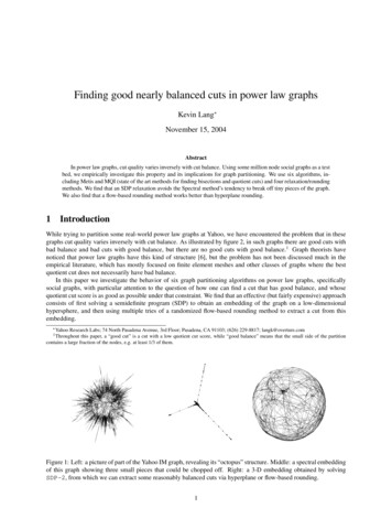
Cuts in a Social Graph (1.9 million nodes from the Yahoo IM Graph)10.9Spectral FlowRounding0.80.70.60.5SDP2 FlowRounding0.40.3MetisSDP-2 LB0.2MQI0.1008k64k216ksize of small side (cube root scale)512k1000kFigure 2: This scatter plot of cuts in a 1.9 million node social graph shows an inverse relationship between cut quality(as measured by quotient cut score) and balance (as measured by the size of a cut’s small side).1.1Some examplesFirst let us consider figure 1-A, in which a small 7287-node piece of the Yahoo IM graph (see section 7) is pictured. Asdiscussed by Chung and Lu in the theoretical paper [6], it is clear that this graph has an “octopus’ structure consistingof many tentacles growing out of a densely connected core. The tentacles provide many opportunities to make highlyunbalanced cuts that have a good quotient cut score. On the other hand, cutting the graph into two large pieces wouldrequire cutting through the high-expansion core, and the many edges that would necessarily be cut make it impossiblefor the quotient cut score to be very good in that case (see also [8]).An inverse tradeoff between cut quality and balance appears clearly in figure 2, which contains a scatter plot ofcuts in a 1.9 million node subgraph of the Yahoo IM graph. The y-axis shows the quality of each cut as measured byits quotient cut score (cutsize / nodes in small side). Smaller quotient cut scores are better. The x-axis shows balanceas measured by the number of nodes on the small side of a cut. The least balanced cuts appear on the left, and the mostbalanced cuts appear on the right.The numerous dots in the lower left corner of figure 2 show that there are many good cuts which unfortunatelyhave terrible balance. On the other hand, there are no dots in the lower right corner, so apparently there are no goodcuts with good balance. To eliminate the possibilty that such cuts exist but are just very hard to find, we have alsoplotted an SDP-based lower bound on balanced cuts.We have also examined a completely different social graph which encodes co-authorship among 136,785 computerscientists, as determined by the DBLP database. The scatter plots in Figure 8 show that the cut structure of this graphhas a strong qualitative resemblence to that of the Yahoo IM graph.2Relaxations of the graph bisection QIPBy adopting a mathematical programming viewpoint and considering various relaxations of the standard Quadratic Integer Program (QIP) for graph bisection, it is possible to discuss most of the theoretically important graph partitioningalgorithms (including the spectral method [16], the multicommodity flow approach of Leighton and Rao[15], and theSDP-based method of Arora, Rao, and Vazirani [17]) in the single framework shown in figure 3.The graph bisection QIP and the three SDP relaxations shown here have all use n indicator variables xi whichbasically assign the graph’s nodes to different sides of the cut. They all have the same objective function 1/4xT Lx(where L is the graph’s Laplacian matrix) which works out to be equal to (or a lower bound on) the number of edges2
SDP 2 "Vector Relaxation"SDP 1 "Spectral Relaxation"Like SDP 1, butrelaxnxi in Rmins.t.14xT LxxTe 0SDP 3relaxrelax(xi * xi ) 1,AMinbis QIPi14xTLxxTe 01xi in R(x i * x i) nmins.t.quadratic U.B.Like SDP 2, butwithineqs.Goemans, Williamsonx i in { 1,1}Fiedler; Alon et alLPO(sqrt(log n))Goemans;Arora, Rao, VaziranimulticommodityflowrelaxO(log n)Leighton RaoFigure 3: Four relaxations of the minimum bisection QIP, three of which correspond to algorithms with theoreticalapproximation guarantees. In this empirical paper we focus on SDP-1 and SDP-2.in the cut defined by the indicator variables. They also include the constraint xT e 0 (where e is a vector of all ones)which encodes the requirement that the solution be balanced,The crucial difference between the QIP and the SDP relaxations lies in the set of values that the indicator variablesxi are allowed to assume. In the case of the original QIP, they are restricted to the set { 1, 1}, where the two valuesdirectly encode the two sides of the cut. Unfortunately, solving the QIP is exactly equivalent to optimally bisecting thegraph, which makes it NP-hard.In SDP-1, the indicator variables can assume arbitrary real values, provided that their average squared magnitudeis 1.0. It has been known for at least 30 years that the solution to SDP-1 is the eigenvector corresponding to thesecond smallest eigenvalue of the graph’s Laplacian matrix [7]. Hence solving SDP-1 is generally known as thespectral method. In the mid 1980’s it was proved by Alon and Milman [1] and other that the spectral method yieldssolutions that are at worst quadratically bad (see also [16]). Later analysis by Spielman and Teng showed why thespectral method works especially well on planar graphs and meshes [19]. On the empirical side, many people over theyears have found that the spectral method works well on various classes of graphs that are of practical interest [18].Unfortunately, when the spectral method is applied to the power law graphs that are the subject of this paper, itwants to break off tiny pieces of the graph. This effect is clearly visible in the middle picture of figure 1, which showsan embedding of our small social graph based on the first three non-trivial eigenvectors of its Laplacian matrix.2How can it be that these spectral solutions are so unbalanced, given that SDP-1 is a relaxation of a QIP for thegraph bisection problem? The reason is illustrated by the see-saw in figure 4. Because the spectral relaxation allowsindicator variables to assume values with widely differing magnitudes, it is possible for a small number of nodes tomove a long ways out from the pivot point at the origin, where they acquire enough leverage to balance a large numberof nodes on the other side.To obtain a more balanced cut, we need to somehow prevent indicator variables from adopting large values andthereby gaining unfair leverage. Obviously we can do this by reverting to our original requirement that every legalindicator value have exactly the same magnitude. However, this takes us back to the original QIP, which is not solvable.Fortunately, there is a brilliant way to escape this apparent dilemma, an idea which was brought to the attentionof the CS community by the Max Cut algorithm of Goemans and Williamson [10]: if we allow the indicator variablesto assume values that are n-dimensional vectors, rather than scalars, then the program remains solvable even with thestrict requirement that every vector has squared length 1.0. We will call this semidefinite program SDP-2. Figure1-C shows what a solution (in 3 rather than n dimensions) to SDP-2 looks like for our small example graph. Theimportant point is that unlike in the spectral solution, small pieces are not being singled out for excision.While solutions to SDP-2 aren’t anything as simple as eigenvectors, we can find them using one of many SDPsolvers, notably Helmberg and Rendl’s program SBmethod [12], and Burer and Monteiro’s special-purpose solverfor SDP-2 which can handle graphs with more than a million nodes [4].2 We frequently hear the suggestion that Malik and Shi’s “normalized cut” version of the spectral method would solve this problem of unbalancedsolutions. It does not, and in fact, figure 1-B was drawn using using normalized cut eigenvectors.3
Desired behaviorBehavior of SDP 1 (spectral relaxation)Figure 4: Because the spectral relaxation (SDP-1) only requires the squared magnitude of indicator values to be 1.0on average, a few nodes can move far from the origin, where they acquire enough leverage to balance everyone else.SDP-2 addresses this problem by requiring the magnitude of each indicator variable to be 1.0.It has been conjectured (for example by Goemans in [9]) that it might be possible to prove a constant factorapproximation guarantee for SDP-3, which addresses another problem of the Spectral method by imposing triangleinequalities on the squared distancesbetween node positions (see figure 9). In a breakthrough paper [17], Arora, Rao, and Vazirani proved an O( log n) approximation ratio for this relaxation, which is the best yet for any graphpartitioning algorithm. However, there are n3 triangle inequalities in SDP-3, so it is not practical to solve it exceptfor very small graphs.3Solving SDP-2 for large graphsThe standard trick for solving a problem like SDP-2 is to perform a change of variables to an n n Gram matrix Gcontaining all pairwise dot products of the indicator vectors xi . This creates a mostly linear problem 1TminL G : diag(G) e, e Ge 0, G 04where the extra constraint G 0 requires G to be positive semidefinite, so that we can factor it to get back tothe indicator vectors that we really want. While this trick has enabled numerous small applications of semidefiniteprogramming, it does have the problem that G is dense and contains n2 entries, which imposes a severe limit on thesize of problems that can be solved.To avoid this barrier to scaling, Burer and Monteiro have taken the surprising step of not doing the standard changeof variables to linearize the problem [4]. Instead, they use non-linear programming techniques to solve the originalquadratic program on the indicator vectors, which are however constrained to be of some much lower dimensionr n. That is, they solve the following non-linear optimization problem over the space of n r matrices R. 1minL RRT : diag(RRT ) e, eT RRT e 04This approach is exploiting a theorem which states that because SDP-2 only has about n constraints, the indicatorvectors do not need more than about n dimensions, so the search space only needs n1.5 rather than n2 degrees offreedom.3 In fact, Burer and Monteiro’s implementation of this idea, SDP-LR, starts with indicator vectors of an evensmaller dimensionality and gradually creeps up on n dimensions if they seem necessary. We have slightly modifiedtheir code4 to use indicator vectors of a very small fixed dimension, like 4 or 8. This means that all theoreticalguarantees are gone, but our ability to handle very large graphs is improved, and in fact we have obtained lowdimensional embeddings of graphs with as many as 2.5 million nodes. This is several orders of magnitude largerthan the graphs that one can handle with the standard approach of using a general purpose SDP solver to find a GramMatrix.Because we do not know the right dimensionality for a given graph’s indicator vectors, we typically try severalpossibilities and compare the resulting objective function values. If, for example, 4 dimensions yields a value that issignificantly higher than the value for 5 dimensions, then 4 dimensions apparently are not enough. On some standardmesh-like benchmark graphs, this approach seems to recover the true dimensionality. Furthermore, on several graphs3 In[3] Burer and Monteiro discuss this issue in detail and also explain why their approach does not get stuck in local minima.we used the special purpose program minbis which is part of SDP-LR v0.130301; the later package SDPLR-1.0 is a generalpurpose solver that does not seem to scale as well.4 Specifically,4
that weren’t too big (with say 50,000 nodes) we have used a complete different solver, namely SBmethod, to findlow-dimensional solutions. This program seems to recover a similar dimensionality, and the objective function valuesand solutions look similar to those that we obtain with SDP-LR. Therefore we believe that the apparently radicallow-rank solutions make some sense.4Two Rounding MethodsA rounding method is needed to convert the graph embedding which results from solving SDP-1 or SDP-2 into aspecific cut. We have tested two rounding methods, both of which are widely applicable and should work on anylow-dimensional embedding of a graph in which the nodes are generally spread out except that nodes connected byedges are close together.4.1Rounding with Swept Random HyperplanesThis method combines two well known ingredients. The first is the “sweep” method commonly used in spectralpartitioning to convert a 1-d embedding of the graph (i.e. an eigenvector) into a specific cut. The embedding impliesan ordering of the nodes, which in turn suggests n 1 obvious possible cuts (namely the first k nodes versus the lastn k nodes, for all 0 k n). By using incremental score updates, in linear time we can “sweep” through thesen 1 cuts, evaluating them all, and then finally we can choose the cut that achieves the best score.The second ingredient is the random hyperplane method that Goemans and Williamson used to round their multidimensional vector relaxation of Max Cut [9]. Here, one chooses a randomly oriented hyperplane through the origin,and then assigns the nodes embedded on either side of that hyperplane to the two sides of the cut.In the SRH rounding method, we choose a randomly oriented hyperplane just like Goemans and Williamson, butinstead of leaving it sitting at the origin, we sweep it (in the direction of its defining unit vector) through the multidimensional graph embedding, evaluating n 1 different cuts just like we did when rounding the 1-d spectral solution.In fact, we do multiple tries, as follows:1. Choose a randomly oriented unit vector u.2. Project the multi-dimensional embedding of the graph onto the line defined by u, and sort the nodes according to this new1-d embedding.3. In linear time, evaluate the n 1 cuts implied by this ordering, and choose the best one.4. If enough directions have been tried, output the best cut that we saw in any iteration. Otherwise, go to back step 1 and try anew direction.4.2Rounding with Maximum FlowAs with SRH, we do multiple tries trying to find a good cut perpendicular to various random directions. Instead ofcutting with a simple hyperplane, we now use flow to search for a minimum S-T cut in each direction. In the following,β is a minimum balance parameter whose value is something like 1/3.1. Choose a randomly oriented unit vector u.2. Project the multi-dimensional embedding onto the line defined by u, and sort the nodes according to this new 1-d embedding.3. Use this ordering to divide the nodes into 3 sets F, M, and L, with F containing the first βn nodes, L containing the last βnnodes, and M containing the remaining nodes, which lie in the middle.4. Set up an S-T max flow problem where the nodes in F are pinned to the source and the nodes in L are pinned to sink byinfinite capacity arcs, and every graph edge generates two arcs, one in each direction, with unit capacity.5. Solve this flow problem to obtain an S-T min cut, which becomes the answer for this iteration. Note that we have explicitlyminimized the cut size, while the balance is reasonable because each side contains at least βn nodes.6. If enough directions have been tried, output the best cut that we saw in any iteration. Otherwise, go to back step 1 and try anew direction.This flow problem construction seems pretty obvious and is probably folklore; something like it is described in [2].We solve the flow problem using hi pr, Cherkassky and Goldberg’s implementation of the highest-node variant ofthe push-relabel algorithm [5]. Its worst case run time is O(n2.5 ), but it seems to run in nearly linear time in practice,with a very good constant factor.5
100000Solving SDP-2 with SDP-LRSolving SDP-1 with ARPACKBisecting graph with MetisSolving flow problem with hi pr10000run time (seconds)10001001010.10.01100100010000100000graph size (nodes edges)1e 061e 07Figure 5: Run times of several algorithms on various subsets of the Yahoo IM graph.5Discussion of run timesFigure 5 plots the growth rate of run time for various programs that we use to solve SDP-1, SDP-2, and the flowproblems which arise during rounding. The test graphs are subsets of the Yahoo IM graph, whose sizes cover fourorders of magnitude. We show times for two solvers for SDP-1, both of which use ARPACK to find three eigenvectorsof the input graph’s Laplacian.5 The solver for SDP-2 is a slightly modified version of Burer and Monteiro’s SDP-LR,which finds an embedding of the graph on the 3-sphere (which lives in 4-space). Surprisingly, this solver for SDP-2runs in a time that is roughly similar to that of the spectral solvers for SDP-1, and for this family of graphs, the growthrate is roughly linear.Run time for the flow problem solver hi pr also grows roughly linearly, but with a constant factor that is 3 ordersof magnitude lower. It seems reasonable to consider that the expense of solving the SDP “pays for” numerous triesduring the rounding phase.For some additional perspective, we have also plotted the run time of Metis on these graphs, which also growsalmost linearly with graph size with a very small constant factor. We note that the MQI method for improving quotientcuts also uses hi pr to solve flow problems, and is also very fast.6The DBLP collaboration graphIn this experiment we tried six algorithms on a non-proprietary graph constructed from the DBLP database of computerscience papers and authors. This graph contained one node for each author, and edges between people who were coauthors on any 2- or 3-author paper. From this raw graph we extracted the largest connected component to obtain agraph with 136,785 nodes and 238,754 edges.All six of the algorithms are randomized. Their outputs are distributions of cuts that are shown in the scatter plotsof Figure 8. Recall that these plots display cut quality (quotient cut score) as a function of balance (size of small side).The red dots on the right side of the figure represent bisections obtained from several hundred runs of a randomizedversion of Metis. These cuts have perfect balance. They have a range of quotient cut scores, but none of them aremuch below 0.15. An approximate lower bound based on the value of the SDP-2 relaxation6 shows that there are infact no bisections with a quotient cut score below about 0.07.The red dots trending down into the lower left of the figure represent cuts that result from using MQI to postprocess the Metis bisections. The lowest and leftmost cut is a 1/60 cut that cuts 1 edge to remove a 60-node tentacle.5 These two programs use ARPACK in different ways. The slower program uses a fixed number (10) of Arnoldi vectors and runs until convergence. The faster program starts with 10 Arnoldi Vectors, but it repeatedly starts over with 10 more if it fails to converge in some number ofiterations. Also, the faster program is computing “normalized cut” eigenvectors, which possibly converge faster.6 Observe that the spectral (SDP-1) bound also plotted in the figure is much worse than the SDP-2 lower bound. We conjecture that this istypical for power law graphs.6
The green dots in figure 8-A represent cuts that were obtained using Spectral plus Swept Hyperplane Rounding. AnARPACK-based program was used to find the lowest three non-trivial eigenvectors of the graph’s Laplacian Matrix.Considered individually, these three eigenvectors recommend that we make a 1/60 cut, a 1/49 cut, and a 1/37 cutrespectively. When considered together as a 3-d embedding and fed into the SRH rounding procedure, we get thesesame cuts plus some other very unbalanced cuts, all of which appear in the lower left corner of the figure. Out ofcuriousity about what other cuts could be possibly be extracted from this embedding using hyperplanes, we modifiedthe rounding program to output several local minima in addition to the true minimum of each sweep. This generatedthe full range of cuts shown by green dots in the figure. Except for the cuts in the lower left corner that Spectral wasactually trying to recommend, none of these cuts are as good as those obtained more cheaply using Metis and MQI.The blue dots in figure 8-A show cuts that were obtained using SDP-2 plus Swept Hyperplane Rounding. TheSDP-2 solutions were obtained using a 5-dimensional version of SDP-LR.7 As before, we used a rounding programthat outputs the true minimum plus some local minima from each sweep. The results are qualitatively different fromthose we obtained from the spectral relaxation. On the unbalanced left-hand side of the plot, SDP-2 is losing toSpectral, while on the balanced right-hand side of the plot, SDP-2 is beating Spectral. However, it is still not doingas well as Metis.Now let us consider the plots in figure 8-B, where the Spectral and SDP-2 solutions are rounded using the flowbased method.8 The resulting cuts are distinctly better than those obtained with the Swept Random Hyperplanerounding. The relative merits of Spectral and SDP-2 are the same as before, with Spectral looking better on the left,and SDP-2 looking better on the right, but now both of them are producing cuts that don’t look bad compared to theMetis and MQI cuts. In fact, SDP-2 plus flow-based rounding has produced some nearly balanced cuts with scoresthat beat those of the Metis bisections.7The Yahoo IM graphThe “Yahoo IM” graph contains nearly 200 million nodes and 800 million edges, and was constructed from the buddylists of users of the Yahoo Instant Messenger service (all completely anonymized). Because this graph is so huge, wetypically use subgraphs obtained by subsampling and/or partitioning. The embeddings pictured in figure 1, and therun times plotted in figure 5 are based on such subsets of the IM graph.Figure 7 contains scatter plots generated by experiments that were just like the DBLP experiments described insection 6 except that they were run on a 1.9 million-node subgraph of the Yahoo IM graph. Clearly, these results havea very strong qualitative resemblence to the results for the DBLP graph. In fact, we can repeat all of the observationsmade earlier, and have done so in the caption to figure 7. In addition, we have used a cube-root scale (analogous to alog scale) for the x-axis here because it reveals a distinct linear pattern that might be of interest to theoretists who aretrying to make models of social graphs. This pattern shows the cut size growing as the 43 power of the number of nodeon the small side of the cut.Because the cut distributions (and algorithm behaviors) that we have observed for these two social graphs areso similar, and so different from what we have seen on some more traditional graphs (especially planar graphs, F.E.meshes, and “geometric graphs”), we conjecture that they are characteristic of social graphs, and possibly of powerlaw graphs in general.8Other classes of graphsThe main topic of this paper is graphs that have an inverse relationship between balance and cut quality. Many classesof graphs do not have this property. To illustrate how that case is different from the one that we have been discussing,we consider a meshlike graph built from an image [picture omitted to save space, but it is a downward-looking viewof some clouds over some mountains.]Once again we used Metis and MQI to obtain an initial idea of the cut structure of the graph. These are shown byred dots in the scatter plots of figure 6-left. Clearly there are no cuts in the lower left corner of the plots; unlike in thecase of power law graphs, here the best quotient cuts have reasonable balance.7 Variousdimensions gave the following objective function values: 3d 4351.0, 4d 4227.1, 5d 4215.5, 6d 4216.5.the interest of filling out the scatter plot, we again slightly modified the rounding procedure. Instead of always using a large β value like0.33, we used random values ranging from 0.001 to 0.499. We point out that the flow problem construction makes less sense for smaller β valuesbecause cut size becomes a very poor approximation of quotient cut score.8 In7
Now we consider cuts found by solving SDP-1 and SDP-2 (green and blue dots) and then applying hyperplaneand flow-based rounding (left and right plots). Apparently, the behaviors of SDP-1 and SDP-2 are not so different inthis case, but the choice of rounding method is still significant. When swept random hyperplane rounding is used, wedo not find the best cuts that we earlier obtained with Metis MQI. However, either SDP-1 or SDP-2 with flow-basedrounding is able to find these cuts.8.1Some traditional benchmark graphsChris Walshaw maintains a website called the “The Graph Partitioning Archive”9 which keeps track of the best nearlybalanced cuts ever found for a number of classic benchmark graphs, with a particular emphasis on FE meshes. Whenwe first checked this site in Spring 2004, very few of the record cuts had been found using the spectral method. Wesuspect that this is due to the weakness of the usual rounding methods, because we discovered that Spectral plus flowbased rounding can find several cuts that would have been new records. Now we have posted some new recordcuts (for the graphs data, wing nodal, t60k, brack2, fe tooth, fe rotor, 144, wave, andauto) that we obtained with SDP-2 plus flow-based rounding, and these may have filled the niche that Spectralplus flow could have occupied.Appendix: Metis and MQIMetis [13] is a high quality implementation of the multi-resolution graph partitioning approach that was found to bevery effective during the 1990’s. It constructs a hierarchy of lower-resolution versions of the graph by repeatedlycontracting the edges of large matchings. At the bottom level a reasonable bisection is found and then brought backup through the hierarchy and refined at each level using local search.MQI [14] is an exact flow-based method (using a different flow problem from the one in this paper) for improvingquotient cuts. Given a quotient cut as input, it tells whether there exists any better quotient cut whose small side is asubset of the input’s small side. If one or more such improved quotient cuts exist, it returns one of them.References[1] N. Alon and V.D. Milman. λ1 , isoperimetric inequalities for graphs, and superconcentrators. Journal of Combinatorial Theory, Series B, 38:73–88, 1985.[2] Yuri Boykov, Olga Veksler, and Ramin Zabih. Fast approximate energy minimization via graph cuts. In ICCV(1), pages 377–384, 1999.[3] Samuel Burer and Renato D.C. Monteiro. Local minima and convergence in low-rank semidefinite programming.Technical report, Department of Management Sciences, University of Iowa, September 2003.[4] Samuel Burer and Renato D.C. Monteiro. A nonlinear programming algorithm for solving semidefinite programsvia low-rank factorization. Mathematical Programming (series B), 95(2):329–357, 2003.[5] Boris V. Cherkassky and Andrew V. Goldberg. On implementing the push-relabel method for the maximum flowproblem. Algorithmica, 19(4):390–410, 1997.[6] F. Chung and L. Lu. Average distances in random graphs with given expected degree sequences. Proceedings ofNational Academy of Science, 99:15879–15882, 2002.[7] W.E. Donath and A. J. Hoffman. Lower bounds for partitioning of graphs. IBM J. Res. Develop., 17:420–425,1973.[8] Christos Gkantsidis, Milena Mihail, and Amin Saberi. Conductance and congestion in power law graphs. In Proceedings of the 2003 ACM SIGMETRICS international conference on Measurement and modeling of computersystems, pages 148–159. ACM Press, 2003.9 http://staffweb.cms.gre.ac.uk/ c.walshaw/partition8
scatter pot of cuts in the clouds picture graph0.1quotient cut scorescatter pot of cuts in the clouds picture graphMetis Bisections MQISpectral Sweep RoundingSDP-2 Sweep RoundingMetis Bisections MQISpectral Flow RoundingSDP-2 Flow Round
wants to break off tiny pieces of the graph. This effect is clearly visible in the middle picture of figure 1, which shows an embedding of our small social graph based on the first three non-trivial eigenvectors of its Laplacian matrix.2 How can it be that these spectral solutions are so