WIXLIB

ChapterIntroduction to Time Series1A time series is a set of observations obtained by measuring a single variable regularly over aperiod of time. In a series of inventory data, for example, the observations might represent dailyinventory levels for several months. A series showing the market share of a product might consistof weekly market share taken over a few years. A series of total sales figures might consist ofone observation per month for many years. What each of these examples has in common is thatsome variable was observed at regular, known intervals over a certain length of time. Thus, theform of the data for a typical time series is a single sequence or list of observations representingmeasurements taken at regular intervals.Table 1-1Daily inventory time vel160135129122108150120One of the most important reasons for doing time series analysis is to try to forecast future valuesof the series. A model of the series that explained the past values may also predict whether andhow much the next few values will increase or decrease. The ability to make such predictionssuccessfully is obviously important to any business or scientific field.Time Series DataWhen you define time series data for use with the Forecasting add-on module, each seriescorresponds to a separate variable. For example, to define a time series in the Data Editor, clickthe Variable View tab and enter a variable name in any blank row. Each observation in a time seriescorresponds to a case (a row in the Data Editor).If you open a spreadsheet containing time series data, each series should be arranged in acolumn in the spreadsheet. If you already have a spreadsheet with time series arranged in rows,you can open it anyway and use Transpose on the Data menu to flip the rows into columns. Copyright SPSS Inc. 1989, 20101

2Chapter 1Data TransformationsA number of data transformation procedures provided in the Core system are useful in timeseries analysis. The Define Dates procedure (on the Data menu) generates date variables used to establishperiodicity and to distinguish between historical, validation, and forecasting periods.Forecasting is designed to work with the variables created by the Define Dates procedure. The Create Time Series procedure (on the Transform menu) creates new time series variablesas functions of existing time series variables. It includes functions that use neighboringobservations for smoothing, averaging, and differencing. The Replace Missing Values procedure (on the Transform menu) replaces system- anduser-missing values with estimates based on one of several methods. Missing data at thebeginning or end of a series pose no particular problem; they simply shorten the useful lengthof the series. Gaps in the middle of a series (embedded missing data) can be a much moreserious problem.See the Core System User’s Guide for detailed information concerning data transformationsfor time series.Estimation and Validation PeriodsIt is often useful to divide your time series into an estimation, or historical, period and a validationperiod. You develop a model on the basis of the observations in the estimation (historical) periodand then test it to see how well it works in the validation period. By forcing the model to makepredictions for points you already know (the points in the validation period), you get an idea ofhow well the model does at forecasting.The cases in the validation period are typically referred to as holdout cases because they areheld-back from the model-building process. The estimation period consists of the currentlyselected cases in the active dataset. Any remaining cases following the last selected case can beused as holdouts. Once you’re satisfied that the model does an adequate job of forecasting, youcan redefine the estimation period to include the holdout cases, and then build your final model.Building Models and Producing ForecastsThe Forecasting add-on module provides two procedures for accomplishing the tasks of creatingmodels and producing forecasts. The Time Series Modeler procedure creates models for time series, and produces forecasts. Itincludes an Expert Modeler that automatically determines the best model for each of yourtime series. For experienced analysts who desire a greater degree of control, it also providestools for custom model building. The Apply Time Series Models procedure applies existing time series models—created by theTime Series Modeler—to the active dataset. This allows you to obtain forecasts for series forwhich new or revised data are available, without rebuilding your models. If there’s reason tothink that a model has changed, it can be rebuilt using the Time Series Modeler.

ChapterTime Series Modeler2The Time Series Modeler procedure estimates exponential smoothing, univariate AutoregressiveIntegrated Moving Average (ARIMA), and multivariate ARIMA (or transfer function models)models for time series, and produces forecasts. The procedure includes an Expert Modeler thatautomatically identifies and estimates the best-fitting ARIMA or exponential smoothing modelfor one or more dependent variable series, thus eliminating the need to identify an appropriatemodel through trial and error. Alternatively, you can specify a custom ARIMA or exponentialsmoothing model.Example. You are a product manager responsible for forecasting next month’s unit sales andrevenue for each of 100 separate products, and have little or no experience in modeling time series.Your historical unit sales data for all 100 products is stored in a single Excel spreadsheet. Afteropening your spreadsheet in IBM SPSS Statistics, you use the Expert Modeler and requestforecasts one month into the future. The Expert Modeler finds the best model of unit sales foreach of your products, and uses those models to produce the forecasts. Since the Expert Modelercan handle multiple input series, you only have to run the procedure once to obtain forecasts forall of your products. Choosing to save the forecasts to the active dataset, you can easily exportthe results back to Excel.Statistics. Goodness-of-fit measures: stationary R-square, R-square (R2), root mean square error(RMSE), mean absolute error (MAE), mean absolute percentage error (MAPE), maximumabsolute error (MaxAE), maximum absolute percentage error (MaxAPE), normalized Bayesianinformation criterion (BIC). Residuals: autocorrelation function, partial autocorrelation function,Ljung-Box Q. For ARIMA models: ARIMA orders for dependent variables, transfer functionorders for independent variables, and outlier estimates. Also, smoothing parameter estimatesfor exponential smoothing models.Plots. Summary plots across all models: histograms of stationary R-square, R-square (R2),root mean square error (RMSE), mean absolute error (MAE), mean absolute percentage error(MAPE), maximum absolute error (MaxAE), maximum absolute percentage error (MaxAPE),normalized Bayesian information criterion (BIC); box plots of residual autocorrelations and partialautocorrelations. Results for individual models: forecast values, fit values, observed values, upperand lower confidence limits, residual autocorrelations and partial autocorrelations.Time Series Modeler Data ConsiderationsData. The dependent variable and any independent variables should be numeric.Assumptions. The dependent variable and any independent variables are treated as time series,meaning that each case represents a time point, with successive cases separated by a constanttime interval. Copyright SPSS Inc. 1989, 20103

4Chapter 2 Stationarity. For custom ARIMA models, the time series to be modeled should be stationary.The most effective way to transform a nonstationary series into a stationary one is through adifference transformation—available from the Create Time Series dialog box. Forecasts. For producing forecasts using models with independent (predictor) variables, theactive dataset should contain values of these variables for all cases in the forecast period.Additionally, independent variables should not contain any missing values in the estimationperiod.Defining DatesAlthough not required, it’s recommended to use the Define Dates dialog box to specify the dateassociated with the first case and the time interval between successive cases. This is done priorto using the Time Series Modeler and results in a set of variables that label the date associatedwith each case. It also sets an assumed periodicity of the data—for example, a periodicity of 12 ifthe time interval between successive cases is one month. This periodicity is required if you’reinterested in creating seasonal models. If you’re not interested in seasonal models and don’trequire date labels on your output, you can skip the Define Dates dialog box. The label associatedwith each case is then simply the case number.To Use the Time Series ModelerE From the menus choose:Analyze Forecasting Create Models.

5Time Series ModelerFigure 2-1Time Series Modeler, Variables tabE On the Variables tab, select one or more dependent variables to be modeled.E From the Method drop-down box, select a modeling method. For automatic modeling, leavethe default method of Expert Modeler. This will invoke the Expert Modeler to determine thebest-fitting model for each of the dependent variables.To produce forecasts:E Click the Options tab.E Specify the forecast period. This will produce a chart that includes forecasts and observed values.Optionally, you can: Select one or more independent variables. Independent variables are treated much likepredictor variables in regression analysis but are optional. They can be included in ARIMAmodels but not exponential smoothing models. If you specify Expert Modeler as the modelingmethod and include independent variables, only ARIMA models will be considered. Click Criteria to specify modeling details. Save predictions, confidence intervals, and noise residuals.

6Chapter 2 Save the estimated models in XML format. Saved models can be applied to new or reviseddata to obtain updated forecasts without rebuilding models. This is accomplished with theApply Time Series Models procedure. Obtain summary statistics across all estimated models. Specify transfer functions for independent variables in custom ARIMA models. Enable automatic detection of outliers. Model specific time points as outliers for custom ARIMA models.Modeling MethodsThe available modeling methods are:Expert Modeler. The Expert Modeler automatically finds the best-fitting model for each dependentseries. If independent (predictor) variables are specified, the Expert Modeler selects, for inclusionin ARIMA models, those that have a statistically significant relationship with the dependentseries. Model variables are transformed where appropriate using differencing and/or a squareroot or natural log transformation. By default, the Expert Modeler considers both exponentialsmoothing and ARIMA models. You can, however, limit the Expert Modeler to only searchfor ARIMA models or to only search for exponential smoothing models. You can also specifyautomatic detection of outliers.Exponential Smoothing. Use this option to specify a custom exponential smoothing model. Youcan choose from a variety of exponential smoothing models that differ in their treatment of trendand seasonality.ARIMA. Use this option to specify a custom ARIMA model. This involves explicitly specifyingautoregressive and moving average orders, as well as the degree of differencing. You can includeindependent (predictor) variables and define transfer functions for any or all of them. You can alsospecify automatic detection of outliers or specify an explicit set of outliers.Estimation and Forecast PeriodsEstimation Period. The estimation period defines the set of cases used to determine the model. Bydefault, the estimation period includes all cases in the active dataset. To set the estimation period,select Based on time or case range in the Select Cases dialog box. Depending on available data, theestimation period used by the procedure may vary by dependent variable and thus differ fromthe displayed value. For a given dependent variable, the true estimation period is the period leftafter eliminating any contiguous missing values of the variable occurring at the beginning or endof the specified estimation period.Forecast Period. The forecast period begins at the first case after the estimation period, and bydefault goes through to the last case in the active dataset. You can set the end of the forecastperiod from the Options tab.Specifying Options for the Expert ModelerThe Expert Modeler provides options for constraining the set of candidate models, specifying thehandling of outliers, and including event variables.

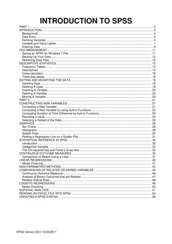
7Time Series ModelerModel Selection and Event SpecificationFigure 2-2Expert Modeler Criteria dialog box, Model tabThe Model tab allows you to specify the types of models considered by the Expert Modeler andto specify event variables.Model Type. The following options are available: All models. The Expert Modeler considers both ARIMA and exponential smoothing models. Exponential smoothing models only. The Expert Modeler only considers exponential smoothingmodels. ARIMA models only. The Expert Modeler only considers ARIMA models.Expert Modeler considers seasonal models. This option is only enabled if a periodicity has beendefined for the active dataset. When this option is selected (checked), the Expert Modelerconsiders both seasonal and nonseasonal models. If this option is not selected, the Expert Modeleronly considers nonseasonal models.Current Periodicity. Indicates the periodicity (if any) currently defined for the active dataset. Thecurrent periodicity is given as an integer—for example, 12 for annual periodicity, with each caserepresenting a month. The value None is displayed if no periodicity has been set. Seasonal modelsrequire a periodicity. You can set the periodicity from the Define Dates dialog box.

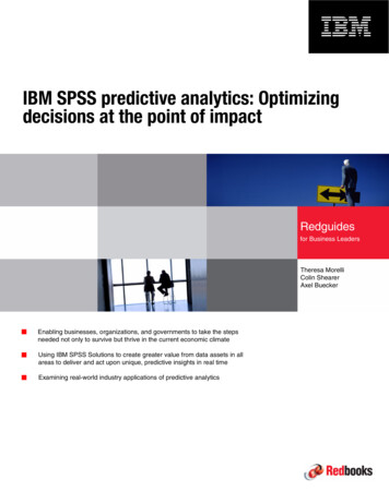
8Chapter 2Events. Select any independent variables that are to be treated as event variables. For eventvariables, cases with a value of 1 indicate times at which the dependent series are expected to beaffected by the event. Values other than 1 indicate no effect.Handling Outliers with the Expert ModelerFigure 2-3Expert Modeler Criteria dialog box, Outliers tabThe Outliers tab allows you to choose automatic detection of outliers as well as the type of outliersto detect.Detect outliers automatically. By default, automatic detection of outliers is not performed. Select(check) this option to perform automatic detection of outliers, then select one or more of thefollowing outlier types: Additive Level shift Innovational Transient Seasonal additive

9Time Series Modeler Local trend Additive patchFor more information, see the topic Outlier Types in Appendix B on p. 94.Custom Exponential Smoothing ModelsFigure 2-4Exponential Smoothing Criteria dialog boxModel Type. Exponential smoothing models (Gardner, 1985) are classified as either seasonal ornonseasonal. Seasonal models are only available if a periodicity has been defined for the activedataset (see “Current Periodicity” below). Simple. This model is appropriate for series in which there is no trend or seasonality. Its onlysmoothing parameter is level. Simple exponential smoothing is most similar to an ARIMAmodel with zero orders of autoregression, one order of differencing, one order of movingaverage, and no constant. Holt’s linear trend. This model is appropriate for series in which there is a linear trend andno seasonality. Its smoothing parameters are level and trend, which are not constrained byeach other’s values. Holt’s model is more general than Brown’s model but may take longerto compute for large series. Holt’s exponential smoothing is most similar to an ARIMAmodel with zero orders of autoregression, two orders of differencing, and two orders ofmoving average. Brown’s linear trend. This model is appropriate for series in which there is a linear trendand no seasonality. Its smoothing parameters are level and trend, which are assumed to beequal. Brown’s model is therefore a special case of Holt’s model. Brown’s exponentialsmoothing is most similar to an ARIMA model with zero orders of autoregression, two ordersof differencing, and two orders of moving average, with the coefficient for the second order ofmoving average equal to the square of one-half of the coefficient for the first order.

10Chapter 2 Damped trend. This model is appropriate for series with a linear trend that is dying out andwith no seasonality. Its smoothing parameters are level, trend, and damping trend. Dampedexponential smoothing is most similar to an ARIMA model with 1 order of autoregression, 1order of differencing, and 2 orders of moving average. Simple seasonal. This model is appropriate for series with no trend and a seasonal effectthat is constant over time. Its smoothing parameters are level and season. Simple seasonalexponential smoothing is most similar to an ARIMA model with zero orders of autoregression,one order of differencing, one order of seasonal differencing, and orders 1, p, and p 1of moving average, where p is the number of periods in a seasonal interval (for monthlydata, p 12). Winters’ additive. This model is appropriate for series with a linear trend and a seasonal effectthat does not depend on the level of the series. Its smoothing parameters are level, trend, andseason. Winters’ additive exponential smoothing is most similar to an ARIMA model withzero orders of autoregression, one order of differencing, one order of seasonal differencing,and p 1 orders of moving average, where p is the number of periods in a seasonal interval(for monthly data, p 12). Winters’ multiplicative. This model is appropriate for series with a linear trend and a seasonaleffect that depends on the level of the series. Its smoothing parameters are level, trend, andseason. Winters’ multiplicative exponential smoothing is not similar to any ARIMA model.Current Periodicity. Indicates the periodicity (if any) currently defined for the active dataset. Thecurrent periodicity is given as an integer—for example, 12 for annual periodicity, with each caserepresenting a month. The value None is displayed if no periodicity has been set. Seasonal modelsrequire a periodicity. You can set the periodicity from

IBM SPSS Statistics is a comprehensive system for analyzing data. The Forecasting optional add-on module provides the additional analytic techniques described in this manual. The Forecasting add-on module must be used with the SPSS Statistics Core system and is completely integrated into that