WIXLIB

Fabietti et al. Brain Inf.(2021) 8:14Page 3 of 19Table 2 Advancements of SANTIA over SigMateToolboxSADUNoCSEUpDFDVSASARFOMFSigMate [15]XXXXSANTIASAD state-of-the-art artifact detection, UNoC unlimited number of channels, SE supported environment, Up updates, DF digital filtering, DV data visualization, SAspectral analysis, SAR stimulation artifact removal, FO file operations, MF multiple formatsan example, the alpha band (8–12 Hz) can have oscillations of high amplitude and be falsely detected as anartifact.There is one other toolbox that deals with LFP artifactdetection. This is SigMate [15–17], a Matlab-based toolthat incorporates standard methods to analyze spikesand electroencephalography (EEG) signals, and in-housesolutions for LFP analysis. The functionality providedby SigMate include: artifact removal, both fast [18] andslow [14], angular tuning detection [19], noise characterization [20], cortical layer activation order detection,and network decoding [21–24], sorting of single trial LFP[25–28], etc. It deals with slow stimulus artifact removalthrough an algorithm that subtracts an estimation of thesignal by averaging the peaks and valleys detected in it,eliminating the offset. In addition, it allows for visualization of the spectrogram using short-time Fourier transform of the recording to allocate artifactual frequencybands and allow their filtering, among many other analysis functionalities.To offer a more competitive toolbox, it has beenexpanded with new functionalities, reported in Table 2.These include state-of-the-art modules for artifact detection, or the analysis of any number of channels unlikeSigMate which is limited to 5. Thus, in this paper, we present the SANTIA toolbox (SigMate Advanced: a NovelTool for Identification of Artifacts in Neuronal Signals),a friendly user interface that aids the offline identificationof artifacts process by simplifying the steps to train powerful computational algorithms with the minimum inputof the user. For a wider adoption by the community, thetoolbox is freely available online at https:// github. com/ Ignac ioFab ietti/ SANTI Atool box.The recording of neuronal data, especially when usingmulti-electrode arrays, can lead to electronic files ofnotable size. Figure 1 illustrates a conducted survey ofthe formats of invasive neural recordings in open datasets [29]. The data show that ‘.mat’ is the preferred extension for storage by a substantial margin. This emphasizesthe necessity to develop tools which address the datasetsavailable in ‘.mat’ format. Therefore, SANTIA was implemented in Matlab and works with single files containing multi-channel data files in a variety of formats. Thetoolbox only depends on the Deep Learning Toolbox andthe basic version of Matlab 2020a and above, thereforecan function in any operating system. SANTIA has beendeveloped with the latest app development environmentof Matlab, which allows it to be supported for longer andbe improved with new modules, such as GUI improvements which are planned for the next update.The remainder of the paper is composed of 5 sections: Sect. 2 describes the local field potentials; Sect. 3describes the methods followed by the testing resultspresented in Sect. 4. Finally, in Sect. 5, discussion andconclusion are presented.2  Local field potentialsLocal field potentials are invasive neuronal recordings,which are equal to the sum of the activity of a neuronalpopulation, that has been low-pass-filtered under 300Hz, and whose amplitude ranges from a few micro-voltsto hundreds of micro-volts or more depending on thestudied structure [30]. They can be recorded by single ormulti-channel micro-electrodes (glass micro-pipettes,metal, or silicon electrodes), during in vitro or in vivoFig. 1 Distribution of formats of local field potential signals in opendatasets, extracted from [29]

Fabietti et al. Brain Inf.(2021) 8:14Page 4 of 19Fig. 2 Recording of extracellular neuronal signals from behaving rodents using linear implantable neural probe (shown in gray). Representativelocal field potential signals with and without movement artifacts are shown from two datasets. The blue traces denote signals without artifacts andthe red traces show examples of movement artifacts present in the signalsexperiments to gain insight into the behavior of brainstructures, and diagnosis, and are used in applicationsuch as brain–machine interfaces. Figure 2 illustrates theconcept.As with all neuronal signals, their recording processcan be influenced by internal and external factors, causing artifacts. Within an organism, electric potentialsare also generated mainly from ocular, muscle, or heart

Fabietti et al. Brain Inf.(2021) 8:14activity, i.e., electrooculogram, electromyogram, andelectrocardiogram, respectively. Examples of externalsources include transmission lines, cellphone signals, andfaulty experimental setup. Local field potentials in particular can be affected by spike bleed-through [31], lightstimulation [32], respiration-coupled oscillations [33],and deep brain stimulation artifacts [34].The consequences of the presence of artifacts can bedetrimental, such as misdiagnosis, disturbance of thestudy of the brain activity, or causing a brain–machineinterface device to be mistakenly operated. Lookingat the case of another neuronal signal, EEG signals, thepresence of abnormalities raised the median review timefrom 8.3 to 20.7 min [35]. To make use of these recording successfully, these artifacts must be first identifiedand then dealt with. The use of computational techniqueswhich are able to learn from complex data patterns hasyielded promising results in the field. In the next section,they will be described.3  Methods3.1  Artifact detectionWhile there are many contributions on artifact detection in neuronal signals, specially non-invasive ones likeEEG, the same cannot be said about LFP. For the latter,the main approach has been the application of ML algorithms in the form of artificial neural networks.Artificial intelligence has been used for analysis of patterns and classification in diverse fields such as, anomalydetection [29, 36–44], biological data mining [45, 46],disease detection [47–58], monitoring of human [59–62],financial forecasting [63], image analysis [64, 65], andnatural language processing [66–68]. Most of the time,these algorithms are composed of multiple layers of neurons for processing of non-linear information and wereinspired by how the human brain works. Each neuroncalculates an inner product of its inputs ( xi ) and theirrespective weights (wi ), and then, the bias (b) is addedand, finally, the non-linear activation function is applied,which in most cases is a sigmoid function, tan hyperbolic, or rectified linear unit. Thus, the output of a neuron ( zi ) can be expressed as detailed in Eq. 1nzi fxi wi b .(1)i 1To propagate the information and train the network, theoutput of a layer is fed as input to the subsequent unit inthe next layer. The result of the final output layer is usedas the solution for the problem.There are many variations of the neural network architecture based on their principles in determining theirrules. For example, authors in [69] trained a multi-layeredPage 5 of 19perceptron (MLP) to identify slow-waves in LFP. An MLPis composed of three sections: an input layer, a hiddenlayer, and an output layer, where the units of the lattertwo use the non-linear activation defined in Eq. 1. Themodeling complex of non-linear relations improves whenit contains multiple numbers of hidden layers, comparedto a shallow architecture [70].In our earlier publications [37], an MLP is employedto identify artifacts in LFP along with two other architectures: long short-term memory (LSTM) networksand one dimensional convolutional neural network (1DCNN) [71, 72]. The diagrams of the main componentsof these architectures are depicted in Fig. 3. The LSTMarchitecture is a type of recurrent network spanningadjacent time steps in a manner that at every point theneurons take the current data input as well as the valuesof the hidden neurons that collect the information of theprevious time steps. On the other hand, convolutionalnetworks are a specific form of neural network that iswell suited to computer vision applications due to theircapacity to hierarchically abstract representations of spatial operations. A variation of it, designed for problemswhere the input is a time sequence, is named 1D-CNN.A comparison of the results obtained can be seen inTable 3. Unlike other machine learning techniques whereexpertise is required to extract significant features fromthe signals and which may cause bias in itself, theseresults indicate that neural networks have the capacityto do it automatically. In addition, it is done in a computationally efficient way: 1-min LFP sampled at 1017 Hzanalyzed in 2.27 s equal 26,881 data points analyzed persecond. As a negative, the training of the neural networkis the step where most time and computational power areconsumed.Having described the classification algorithm that willbe used in the toolbox, we proceed to detail its use in thenext section.3.2  OperationThe toolbox can be directly downloaded from the Githubrepository (https:// github. com/ Ignac ioFab ietti/ SANTI Atool box). Once the toolbox is launched, the GUI provides easy access to all modules. It is important to highlight that SANTIA is a generic environment structuredaround one single interface in which specific functionswere implemented, not a library of functions on top ofwhich a GUI has been added to simplify access.It is structured in three main modules, designed to perform various processing and analysis on the neuronal signal files. The main functionalities of the first one include:data loading, scaling, reshaping, channel selection, labeling, saving, and 2D display. The second module is composed of: data loading and splitting, hyper-parameter

Fabietti et al. Brain Inf.(2021) 8:14Page 6 of 19BACFig. 3 Architectures of different neural network models: multi-layer perceptron (A), long short-term memory (B), and one-dimension convolutionalneural network (C). Each circle represents a neuron, multiple rectangles a layer’s depth, and the arrows how the information is propagatedthroughout each networkTable 3 Performance comparison, extracted from [72]NetworkAccuracyParameters1D-CNN [72]95.1561218MLP [37]93.21532LSTM [71]87.14418Computationaltime (s)2.27 0.132.57 0.063.47 0.04setting, network load or design, network train, test setclassification, and threshold setting and saving. Finally,the third one comprehends: data and network loading,classification, and 2D data display and saving.The GUI allows for user interaction via the selection offunctions, parameters, and keyboard inputs, which areprocessed in the back end. A verification routine executesbefore running any function to ensure the user has notskipped a step or has not completed the necessary inputsor parameter selection. This minimizes the possiblehuman errors and time expenditure. In case of doubt ofthe purpose of an element of the GUI, tool tips appearwhen hovering the cursor over it with a brief explanation.The functions to display warning messages, generatefigures, and compute the labeling, training, or classification are allocated in the back end. These developed features were tested with a dataset recorded from a 4-shank,

Fabietti et al. Brain Inf.(2021) 8:14Page 7 of 19Fig. 4 Screenshots of the SANTIA toolbox graphical user interface: Data Labeling (A), Neural Network Training (B), and Classify New Unlabeled Data(C)

Fabietti et al. Brain Inf.(2021) 8:14Page 8 of 19Fig. 5 Functional block diagram of the Toolbox.Arrows in black correspond to the “Data Labeling” module , in red to the “Neural Network Training”module, in dark blue to the “Classify New Unlabeled Data” module, and the purple arrows indicate the progress output16-contact site electrode from anesthetized rats. Atthe end of each module, the respective outputs can beexported to a ‘.mat’ file, which can easily be utilized inother applications due to the accessibility of the format.The following sections describe the individual modulesin greater detail. As a visual aid, Fig. 4 shows the screenshots of the software package, Fig. 5 illustrates the function block diagram, and finally, Fig. 6 shows the workflowdiagram.3.2.1  Data labelingIn the first module, the process begins with the ‘LoadSignals’ button, which opens the import wizard to loadthe neural recordings as an m n matrix, where m is thenumber of channels and n are the data points of eachchannel signal. The compatible formats include ASCIIbased text (.txt, .dat, .out, .csv), spreadsheets files (.xls,.xlsx, .xlsm), and Matab files (.set, .mat), which correspond to 93% of the surveyed data in Fig. 1. The user isrequired to input the sampling frequency in Hz and thewindow length in seconds that they wish to analyze. Inaddition, the unit of the recording and the opportunity toscale is presented, as lots of errors happen due to incorrect annotations of magnitudes.Once all of these parameters have been filled, ‘GenerateAnalysis Matrix’ will structure the data for posterioranalysis. This means that given a window length w, andsampling frequency f, the m n matrix becomes a new

Fabietti et al. Brain Inf.(2021) 8:14Page 9 of 19Fig. 6 Workflow of the SANTIA toolbox, where the “Data Labeling” modules are colored yellow, the “Neural Network Training” modules in green, and“Classify New Unlabeled Data” modules in bluem np w f and q w f . This is incorp q one, whereporated into a table that has row names that follow theformat ‘file id channel i window j’ where file id isthe name of the LFP data file, i the number of channelswhere i 1, . . . , m and j the corresponding window. Inaddition, its columns are named: first “window power”followed by the values of the signal where k 1, . . . , q .tkAs this process involves the creation of p amount of rownames and window’s power, a memory check is done toread available memory and alert if the usage of more than80% of the available memory would be needed.The option to save these data for posterior classification is presented as ‘Save Unlabeled Data’. Otherwise,the user continues by selecting a channel in the dropdown menu or clicking on a table cell and the ‘ThresholdSelection Table’ process. This opens a new window withthe structured data table, and by clicking on a row, theoptions to plot the selected window or to define its poweras a threshold value appear. As a visual aid, windows withsame or higher power are colored red and those with lessgreen, i.e., artifactual and normal, respectively.In another manner, the user can manually input threshold values in the main app’s table, and once he has completed it for all channels, the data can be labeled andsaved as a standardized struct, which contains the original filename, the structured data with its labels, thesampling frequency, window length, the scale, and thethreshold values. This information allows researchers toquickly identify different matrices they create and wish tocompare. An aid in form of text in the ‘Progress’ bannerallows the users to know when each step has been completed, and it is replicated throughout each module.The user can also structure the data for SigMate analysis. The toolbox expects a datapoints(n) channels(m)format, with the first column as timestamp and each ofthe channel’s signal in the following columns. In addition,

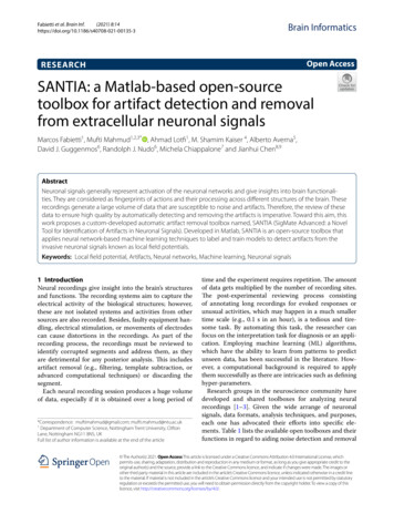
Fabietti et al. Brain Inf.(2021) 8:14Page 10 of 19Table 4 Guide to determine best channels and epochs to use of baseline walk and rest recordings in medial prefrontal cortex (mPFC)and the mediodorsal (MD) thalamus, as mentioned in the file named “Coherence Phase Plot Guide”RatmPFC chan1mPFC chan2MD chan1MD chan2Walk epochRest �2250406080Iteration100 120100 TrainLoss100ms ValAcc255075100 125 15010.90.80.70.60.50.40.30.20.100Loss10.90.80.7150 TrainLoss150ms ValAcc0.60.50.40.30.20.100 20 40 60 80 100 120 140 160IterationLossAccuracy (%) / LossAccuracy (%) / LossIteration200 TrainLoss200ms ValAcc4080120Iteration160200Accuracy (%) / Loss100 200 300 400 500 600Iteration10.90.80.70.60.50.40.30.20.100 50 100 150 200 250 300 350 400Iteration10.90.80.70.60.50.40.30.20.100 20 40 60 80 .100Fig. 7 Training plots for models trained with the first datasetAccuracy (%) / Loss20MLP50 100 150 200 250 300 01001205060IterationAccuracy (%) / Loss50 TrainLoss50ms ValAcc10.90.80.70.60.50.40.30.20.100Accuracy (%) / 80.70.60.50.40.30.20.100LossAccuracy (%) / LossAccuracy (%) / LossThe first column is the rat identification, column 2 and 3 the selected two best channels of the mPFC recordings, and 4 and 5 of the MD recordings. Finally, column 6shows the range of artifact-free epochs during walking and column 7 during resting, respectively [74]10.90.80.70.60.50.40.30.20.100 10 20 30 40 50 60 70 80 90 100Iteration10.90.80.70.60.50.40.30.20.10020 40 60 80 100 120 140 160Iteration

Fabietti et al. Brain Inf.(2021) 8:14as it only handles five channels at a time, m/5 files haveto be generated. Thus, SANTIA transposes the inputmatrix, generates the timestamp based on the declaredsampling frequency, and generates the files. Afterward, itasks the user to select a directory to save them.3.2.2  Neural network trainingThe second module starts with loading structured datafrom the previous module. The user is asked to set thevalues for training, validation, and test splitting. This iscommon practice to avoid over- and under-fitting results.As artifacts are rare events, the datasets usually presentstrong imbalance which can cause bias in the training;a tick box for balancing the data is present next to the‘Split’ button. Clicking it generates three datasets withnon-repetitive randomized elements from the originalmatrix.This is followed by choosing the network, where theoptions are MLP, LSTM, 1D-CNN, or for the user toload his/her custom set of layers. This is done by choosing a Matlab file which has a Layer-type variable, i.e.,layers that define the architecture of neural networksfor deep learning, without the pre-trained weights.These can be modified via console or the Deep NetworkDesigner Toolbox, and for more information, we directthe reader to the mathworks page1. While employing different architectures might yield better results, it is alsopossible that they might not be structured properly andlead to under-fitting, over-fitting, or fail to learn at all.Therefore, a limitation of employing custom networksis the time consumption that takes getting the correctcombination of layers, as well as setting parameters suchas filter size or activation function. Optionally, the usercan customize the training hyper-parameters such asthe solver, initial learning rate, and execution environment, among others. These intentionally mirror the onesincluded in the Deep Network Designer to facilitate itsusage to those familiarized with it. These are removedfor the MLP option, as it uses a different toolbox (i.e.,patternnet of Deep Learning Toolbox [73]), which thusdoes not allow the same configurations. Clicking the‘Create Network” button loads the training options andsets the input layer to match the window size.The ‘Train Network’ button runs the train network function, which inherits the training optionsand network previously defined. For the 1D-CNN, asthe deep learning toolbox is intended for images, the2D matrices are resized to a 4D vector: 1 windowlength 1 number of windows, originally intendedto be: width height channels number of examples.A display of the training process automatically appears,1https:// uk. mathw orks. com/ help/ deepl earni ng/ ref/ nnet. cnn. layer. layer. htmlPage 11 of 19unless the user decides not to, which enables monitoring the process and early stopping.Having completed the training, the user can selectwhether the ‘Classify Test Set’ displays the confusionmatrix, the area under the receiver-operating characteristic (AUROC) curve, or opens up a new windowwhere the accuracy, F1 score, and confusion matrixappear along with the possibility to modify the classification threshold (set at 0.5 by default). Finally, ‘SaveResults’ creates a struct with data’s filename, the trainednetwork, the training information, the test set’s classification threshold, AUROC, accuracy, F1 score, and confusion matrix.3.2.3  Classify new unlabeled dataThe last module begins with loading a trained net alongwith its classification threshold and unlabeled structureddata. After its classification, the options to plot each ofthe windows with the corresponding color-coded labelappear. Finally, users can save the labels as a table withthe corresponding window name. Having described thetoolbox’s methods, components, and its functions, weproceed to a test case with real recorded LFP.4  ResultsIn this section, we describe the datasets used to test theapp, and the results obtained from them. The artifactdetection task

is a toolbox intended for spectral analysis of continuous neural time series data recorded simultaneously from multiple sensors. It is composed mainly of tools for auto-regressive model estimation, spectral quantity analysis, and network analysis. All functionality has been inte