WIXLIB

ESE250Lab 5: Nyquist-Shannon Sampling TheoremSpring 2013University of PennsylvaniaDepartment of Electrical and Systems EngineeringDigital Audio BasicsESE250 Spring 2013Lab 5: Nyquist-Shannon Sampling Theorem Thursday, February 10, 2011For Lab Session: Tuesday, February 15, 2011 in Ketterer Lab.Due: Monday, February 21, 2011 by 12:00pm.Collaboration: Work in lab in teams of 2. Perform individual writeups. See course collaboration policy in the Administrative Handout.Objective: Appreciate and experience sampling rates; understand aliasing.Prelab Requirements: Download and read this entire lab assignment especially the Motivationsection and the Theory subsection of the Lab Writeup Guidelines section. Bring your headphones. Optional but highly encouraged, encode a track from one of your music CDs into a .wavfile sampled at 48KHz, 16bits.1Deliverable: Names of all lab group members Answers to all lab questions (including prelab question) Your version of generalSampling.viHandin: All labs will be turned in electronically through the Penn Blackboard website. Go to theassignment submission link and follow the instructions. Please submit all your files as one zip file.Also, remember that your writeup should be a PDF file.Exit Ticket: Play for your TA an under-sampled version of your voice recording.1Make sure you encode it from a CD, re-encoding an existing .mp3 into a .wav will not be useful for the lab.1

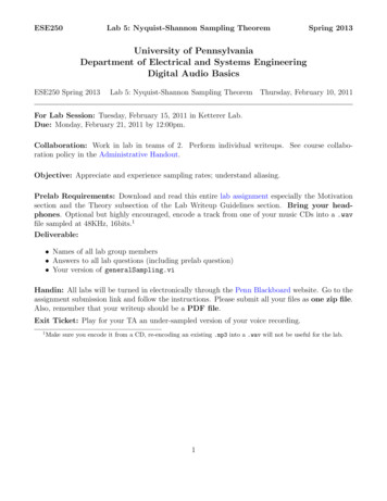
ESE250Lab 5: Nyquist-Shannon Sampling TheoremSpring 2013MotivationWhen sampling, we must take care to ensure that we are sampling at the right frequency to preventaliasing (a phenomenon that occurs when you sample at a lower frequency than is needed). In thislab you will investigate the relationship between the sampling rate and the frequency content of thesound to be sampled. You will look at aliasing, how it affects sampled waves, and how to preventaliasing.Lab ProcedureSampling Pure TonesIn class we did a group exercise where our sampling rate was not high enough to capture the trueform of the signal. In this part of the lab you will be able to experiment with different frequenciesand sampling rates and see, first hand, why aliasing happens. To better exhibit the effects, theoriginal signal will only be pure tones. Make sure you have a copy of lab5.zip unzipped and load toneSampling.viFigure 1 shows the front panel for toneSampling.vi. On the left you have the controls that let youadjust the frequency of the signal we want to capture (Frequency of the Signal to be Acquired) aswell as the Sampling Frequency at which you will sample points from the original signal. You canalso play the original signal and the sampled signal and see what is the ratio of sampling frequencyto signal frequency.On the right you will find three graphs. The top graph shows the time domain of the original signal(in thin blue lines) and the sampling points (black points) and linearly interpolated curve they form(in thick black dotted lines). The bottom left graph shows the same time domain view but over amuch shorter time period so that you can more easily see the details of what is happening whenyou go to high frequencies. The last graph, lower right, shows the frequency response of the originalsignal (blue spike) as well as the perceived frequency of the sampled signal (black spike). Double-click on toneSampling.vi to open the VI in LabView Run the VI and see and hear how the signals change as you change both slidersFOR QUESTIONS:1. Set the signal frequency, f , to 440Hz.2

ESE250Lab 5: Nyquist-Shannon Sampling TheoremSpring 2013Figure 1: Sampling pure tones2. Record the minimum sampling rate at which you no longer experience aliasing.3. At this sampling rate, find the ratio R of the sampling rate to the signal frequency f .4. Change the signal frequency f and repeat steps 2 and 3 (try some higher and some lowerfrequencies).5. Once you’ve tried a few different values, fix your signal frequency f at a value of your choice.6. Adjust your sampling rate toLess than fEqual to fGrater than f , but less than f RGreater than f R7. Observe what happens to the look and sound of the wave when you adjust the samplingfrequency.Aliasing NoiseAliasing noise happens when the original signal has information at higher frequencies than thesampling frequency. The sampling operation causes these high frequencies to be aliased to lowfrequencies, where they cause unwanted interference or noise. Getting rid of this noise requires usto apply an anti-aliasing filter before sampling the signal. Since the aliasing noise comes from highfrequencies, the anti-aliasing filter that we use is a low-pass filter.3

ESE250Lab 5: Nyquist-Shannon Sampling TheoremSpring 2013An ideal low-pass filter allows all frequencies below a specified frequency to pass and completelyremoves any frequencies above the specified frequency. This allows us to get rid of the part of thesignal that would otherwise be aliased and produce noise. Load AliasingNoise.vi and run it.With AliasingNoise.vi you will be able to simulate the effect of noise aliasing into the signal.Figure 2 shows the front panel of this VI. As with the previous VI, the left side is the controls andthe right side shows graphs of the signal in the time and frequency domains. The controls allowyou to specify the frequencies of both the signal and the noise, set the sampling rate and define thecutoff frequency for the low-pass filter. You can also listen to the filtered and unfiltered signals.The three rightmost graphs are frequency domain graphs of the filtered and unfiltered signals aswell as the difference between the two, showing which frequencies were removed by the filter. TheGraph Key in the middle of the VI explains what each frequency marking on the graph is. Greenand black dotted lines show the frequencies for the filter and sampling rate. The blue lines representthe signal, bright blue for the specified frequency in the controls and light blue if there is an aliasedfrequency. The frequency of the noise is marked by a red line, again bright red for the specifiedfrequency in the controls and light red if there is aliasing.The final two graphs, Filtered Time and Unfiltered Time, show the filtered and unfiltered signalsin the time domain. You can zoom in and out of these graphs to examine how the signals changeas you change the controls.When you first run the VI, it will show a signal of 400Hz and noise at 3,300Hz. You will also seethe noise aliasing to 300Hz and the filter, at 600Hz removing the noise and aliased noise and leavingthe signal intact.As you change the sliders in the control, you may notice that the Error lights light up on the Signaland Noise controls, you should ignore any effects you see when this happens and change the slidersby 1Hz to get rid of these errors. The error is due to an internal LabView VI.FOR QUESTIONS: Leaving the default values:1. Observe how the filtered and unfiltered signals differ, both visually and audibly.2. Lower the noise frequency until it no longer aliases. Record the noise frequency at which thishappens.3. Keeping the noise to the frequency discovered in the previous question, adjust the frequencyof the low-pass filter to the maximum frequency you can set the filter to before you see noisein the Filtered graphs. Record that frequency4. Rounding to the nearest whole number, find the ratio of the sampling rate to the filter frequency4

ESE250Lab 5: Nyquist-Shannon Sampling TheoremSpring 2013Figure 2: Aliasing noisePick new values for the four sliders so that they meet both of the following requirements: fsignal flow pass fnoise fsampingRate 2 fsignalWrite down the new values and repeat steps 2 to 4 for these new values.Signal ReconstructionFrom lecture and the last two sections you know that if you set the sampling frequency correctlyand filter your signal you can perfectly capture your signal up to the Nyquist frequency. Eventuallyyou will want to reconstruct the analog signal from the sampled points. However, as you will seein this section, simply “connecting the dots” will not produce the original signal faithfully. Load reconstructSignal.vi and run it.This VI (Figure 3) shows two different ways of reconstructing the sampled signal. It lets you specifya frequency of the original signal as well as the sampling frequency. Both graphs show the sampledpoints. The top graph shows the signal obtained by joining the sampled points with a straight line.5

ESE250Lab 5: Nyquist-Shannon Sampling TheoremSpring 2013The bottom graph shows what the correct reconstruction looks like. It does this by first convertingthe time domain samples into the frequency domain using a DFT and then using the frequenciesdiscovered, it reconstructs the time signal by combining the frequencies (similar to what you did tosimulate instruments in lab4).Figure 3: Signal reconstructionSet the frequency and sampling frequency to the ratio you learned in class and discovered in sectionSampling Pure Tones of this lab.FOR QUESTIONS: Observe how the two types of reconstructions look and sound. Find the sampling rate you need to make the “connect the dots” wave sound and look likethe reconstructed wave when frequency is set to 440Hz. Record the ratio between this sampling rate and the frequency. Vary the frequency and find the ratio for a number of different frequencies.Sampling Arbitrary SignalsNow that you understand what is required for successful sampling and signal reconstruction, youwill build a simple VI that lets you sample and reconstruct arbitrary signals stored in a .wav file.6

ESE250Lab 5: Nyquist-Shannon Sampling TheoremSpring 2013If you brought an encoded piece of music, make sure you have it handy, if not, download one of the.wav files from Blackboard.We will also make a voice recording that you will use as another sample signal. To do this, we willneed to use recorder.vi. close LabView completely. Connect the microphone to the computer. Load recorder.vi but don’t run it.This VI lets you set a recording length and a file path where you want to store your recordings.When you run it, it will record from the microphone and display the recorded signal on the graph. As you create recordings, you may find it necessary to adjust the recording volume as explainedbelow.– Right click on the speaker icon in the bottom right of the screen– Click on Open Volume Control– Select Options Properties in the Master Volume window– Make sure Mixer device shows SoundMAX HD Audio– Select Recording and click OK– Adjust the volume of the microphone and repeat the previous steps until the signal is nolonger being cut. Record one or two conversations between you and your lab partner.The VI you will build will allow you to choose a .wav file, the sampling and anti-aliasing filterfrequencies, the reconstruction type (connect or reconstruct) and whether to apply the filter or not.It will also play the sampled signal and display it on a graph. The final block diagram for the VIwill look similar to figure 4. Open a blank VI Right click on the front panel and under the Buttons & Switches tab choose a switch thatwill be used to turn the filter on and off. Place it anywhere on your front panel. Again, right click on the front panel and place a Graph from the Graph Indicators tab. Switch to the block diagram ctrl E.7