Transcription
Perceptual Coding of Digital Audio†Ted Painter, Student Member IEEE, and Andreas Spanias, Senior Member IEEEDepartment of Electrical Engineering, Telecommunications Research CenterArizona State University, Tempe, Arizona 85287-7206spanias@asu.edu, painter@asu.eduABSTRACTDuring the last decade, CD-quality digital audio has essentially replaced analog audio. Emerging digital audio applications for network, wireless, and multimedia computing systems face a series of constraints such as reduced channel bandwidth, limited storage capacity, and low cost. These new applications have created a demand for high-quality digital audiodelivery at low bit rates. In response to this need, considerable research has been devoted to the development of algorithmsfor perceptually transparent coding of high-fidelity (CD-quality) digital audio. As a result, many algorithms have been proposed, and several have now become international and/or commercial product standards. This paper reviews algorithms forperceptually transparent coding of CD-quality digital audio, including both research and standardization activities. The paper is organized as follows. First, psychoacoustic principles are described with the MPEG psychoacoustic signal analysismodel 1 discussed in some detail. Next, filter bank design issues and algorithms are addressed, with a particular emphasisplaced on the Modified Discrete Cosine Transform (MDCT), a perfect reconstruction (PR) cosine-modulated filter bank thathas become of central importance in perceptual audio coding. Then, we review methodologies that achieve perceptuallytransparent coding of FM- and CD-quality audio signals, including algorithms that manipulate transform components, subband signal decompositions, sinusoidal signal components, and linear prediction (LP) parameters, as well as hybrid algorithms that make use of more than one signal model. These discussions concentrate on architectures and applications ofthose techniques that utilize psychoacoustic models to exploit efficiently masking characteristics of the human receiver. Several algorithms that have become international and/or commercial standards receive in-depth treatment, including the††ISO/IEC MPEG family (-1, -2, -4), the AT&T PAC/EPAC/MPAC, the Dolby ††††††AC-2 /AC-3 , and the Sony††ATRAC /SDDS algorithms. Then, we describe subjective evaluation methodologies in some detail, including theITU-R BS.1116 recommendation on subjective measurements of small-impairments. The paper concludes with a discussionof future research directions.I. INTRODUCTIONAudio coding or audio compression algorithms are used to obtain compact digital representations of high-fidelity (wideband) audio signals for the purpose of efficient transmission or storage. The central objective in audio coding is to representthe signal with a minimum number of bits while achieving transparent signal reproduction, i.e., generating output audio thatcannot be distinguished from the original input, even by a sensitive listener (“golden ears”). This paper gives a review of algorithms for transparent coding of high-fidelity audio.The introduction of the compact disk (CD) in the early eighties [1] brought to the fore all of the advantages of digitalaudio representation, including unprecedented high-fidelity, dynamic range, and robustness. These advantages, however,came at the expense of high data rates. Conventional CD and digital audio tape (DAT) systems are typically sampled at either 44.1 or 48 kilohertz (kHz) using pulse code modulation (PCM) with a sixteen bit sample resolution. This results in uncompressed data rates of 705.6/768 kilobits per second (kbps) for a monaural channel, or 1.41/1.54 megabits per second(Mbps) for a stereo pair at 44.1/48 kHz, respectively. Although high, these data rates were accommodated successfully infirst generation digital audio applications such as CD and DAT. Unfortunately, second generation multimedia applicationsand wireless systems in particular are often subject to bandwidth and cost constraints that are incompatible with high datarates. Because of the success enjoyed by the first generation, however, end users have come to expect “CD-quality” audioreproduction from any digital system. Therefore, new network and wireless multimedia digital audio systems must reducedata rates without compromising reproduction quality. These and other considerations have motivated considerable researchduring the last decade towards formulation of compression schemes that can satisfy simultaneously the conflicting demandsof high compression ratios and transparent reproduction quality for high-fidelity audio signals†Portions of this work have been sponsored by a grant from the NDTC Committee of the Intel Corporation. Direct all communications to A. Spanias.††“Dolby,” “Dolby Digital,” “AC-2,” “AC-3,” and “DolbyFAX,” are trademarks of Dolby Laboratories. “Sony Dynamic Digital Sound,” “SDDS,” “ATRAC,” and “MiniDisc” are trademarks of SonyCorporation.
[2][3][4][5][6][7][8][9][10][11]. As a result, several standards have been developed [12][13][14][15], particularly in the lastfive years [16][17][18][19], and several are now being deployed commercially [330][333][336][338] (Table 4).A. GENERIC PERCEPTUAL AUDIO CODING ARCHITECTUREThis review considers several classes of analysis-synthesis data compression algorithms, including those which manipulate: transform components, time-domain sequences from critically sampled banks of bandpass filters, sinusoidal signalcomponents, linear predictive coding (LPC) model parameters, or some hybrid parametric set. We note here that althoughthe enormous capacity of new storage media such as Digital Versatile Disc (DVD) can accommodate lossless audio coding[20][21], the research interest and hence all of the algorithms we describe are lossy compression schemes which seek to exploit the psychoacoustic principles described in section two. Lossy schemes offer the advantage of lower bit rates (e.g., lessthan 1 bit per sample) relative to lossless schemes (e.g., 10 bits per sample). Naturally, there is a debate over the qualitylimitations associated with lossy compression. In fact, some experts believe that uncompressed digital CD-quality audio(44.1 kHz/16b) is intrinsically inferior to the analog original. They contend that sample rates above 55 kHz and wordlengths greater than 20 bits [21] are necessary to achieve transparency in the absence of any compression. The latter debateis beyond the scope of this review.Before considering different classes of audio coding algorithms, we note the architectural similarities that characterizemost perceptual audio coders. The lossy compression systems described throughout the remainder of this review achievecoding gain by exploiting both perceptual irrelevancies and statistical redundancies. Most of these algorithms are based onthe generic architecture shown in Fig. 1. The coders typically segment input signals into quasi-stationary frames rangingfrom 2 to 50 milliseconds in duration. Then, a time-frequency analysis section estimates the temporal and spectral components on each frame. Often, the time-frequency mapping is matched to the analysis properties of the human auditory system,although this is not always the case. Either way, the ultimate objective is to extract from the input audio a set of timefrequency parameters that is amenable to quantization and encoding in accordance with a perceptual distortion metric. Depending on overall system objectives and design philosophy, the time-frequency analysis section might contain a Unitary transform Time-invariant bank of critically sampled, uniform or non-uniform bandpass filters Time-varying (signal-adaptive) bank of critically sampled, uniform or non-uniform bandpass filters Harmonic/sinusoidal analyzer Source-system analysis (LPC/Multipulse excitation) Hybrid transform/filter bank/sinusoidal/LPC signal analyzerThe choice of time-frequency analysis methodology always involves a fundamental tradeoff between time and frequencyresolution requirements. Perceptual distortion control is achieved by a psychoacoustic signal analysis section that estimatessignal masking power based on psychoacoustic principles (see section two). The psychoacoustic model delivers maskingthresholds that quantify the maximum amount of distortion at each point in the time-frequency plane such that quantizationof the time-frequency parameters does not introduce audible artifacts. The psychoacoustic model therefore allows the quantization and encoding section to exploit perceptual irrelevancies in the time-frequency parameter set. The quantization andencoding section can also exploit statistical redundancies through classical techniques such as differential pulse code modulation (DPCM) or adaptive DPCM (ADPCM). Quantization can be uniform or pdf-optimized (Lloyd-Max), and it might beperformed on either scalar or vector data (VQ). Once a quantized compact parametric set has been formed, remaining redundancies are typically removed through run-length (RL) and entropy (e.g. Huffman [22], arithmetic [23], or Lempel-ZivWelch (LZW) [24,25]) coding techniques. Since the output of the psychoacoustic distortion control model is signaldependent, most algorithms are inherently variable rate. Fixed channel rate requirements are usually satisfied through bufferfeedback schemes, which often introduce encoding dEncodingEntropy(Lossless)CodingBit AllocationMUXto chan.Side InfoFig. 1. Generic Perceptual Audio EncoderThe study of perceptual entropy (PE) suggests that transparent coding is possible in the neighborhood of 2 bits per sample[101] for most for high-fidelity audio sources ( 88 kpbs given 44.1 kHz sampling). The lossy perceptual coding algorithmsdiscussed in the remainder of this paper confirm this possibility. In fact, several coders approach transparency in the neighborhood of just 1 bit per sample. Regardless of design details, all perceptual audio coders seek to achieve transparent quality2
at low bit rates with tractable complexity and manageable delay. The discussion of algorithms given in sections IV throughVIII brings to light many of the tradeoffs involved with the various coder design philosophies.B. PAPER ORGANIZATIONThis paper is organized as follows. In section II, psychoacoustic principles are described. Johnston’s notion of perceptual entropy [45] is presented as a measure of the fundamental limit of transparent compression for audio, and the ISO/IECMPEG-1 psychoacoustic analysis model 1 is presented. Section III explores filter bank design issues and algorithms, with aparticular emphasis placed on the Modified Discrete Cosine Transform (MDCT), a perfect reconstruction (PR) cosinemodulated filter bank that is widely used in current perceptual audio coding algorithms. Section III also addresses pre-echoartifacts and control strategies. Sections IV through VII review established and emerging techniques for transparent codingof FM- and CD-quality audio signals, including several algorithms that have become international standards. Transformcoding methodologies are described in section IV, subband coding algorithms are addressed in section V, sinusoidal algorithms are presented in section VI, and LPC-based algorithms appear in section VII. In addition to methods based on uniform bandwidth filter banks, section V covers coding methods that utilize discrete wavelet transforms (DWT), discretewavelet packet transforms (DWPT), and other non-uniform filter banks. Examples of hybrid algorithms that make use ofmore than one signal model appear throughout sections IV through VII. Section VIII is concerned with standardization activities in audio coding. It describes recently adopted standards such as the ISO/IEC MPEG family (-1 “.MP1/2/3”, -2, -4),the Phillips’ Digital Compact Cassette (DCC), the Sony Minidisk (ATRAC), the cinematic Sony SDDS, the AT&T Perceptual Audio Coder (PAC)/Enhanced Perceptual Audio Coder (EPAC)/Multi-channel PAC (MPAC), and the Dolby AC-2/AC3. Included in this discussion, section VIII-A gives complete details on the so-called “.MP3” system, which has been popularized in World Wide Web (WWW) and handheld media applications (e.g., Diamond RIO). Note that the “.MP3” label denotes the MPEG-1, Layer III algorithm. Following the description of the standards, section IX provides information onsubjective quality measures for perceptual codecs. The five-point absolute and differential subjective grading scales are addressed, as well as the subjective test methodologies specified in the ITU-R Recommendation BS.1116. A set of subjectivebenchmarks is provided for the various standards in both stereophonic and multi-channel modes to facilitate inter-algorithmcomparisons. The paper concludes with a discussion of future research directions.For additional information, one can also refer to informative reviews of recent progress in wideband and high-fidelityaudio coding which have appeared in the literature. Discussions of audio signal characteristics and the application of psychoacoustic principles to audio coding can be found in [26],[27], and [28]. Jayant, et al. of Bell Labs also considered perceptual models and their applications to speech, video, and audio signal compression [29]. Noll describes current algorithmsin [30] and [31], including the ISO/MPEG audio compression standard. Also recently, excellent tutorial perspectives onaudio coding fundamentals [32], as well as signal processing advances [33] central to audio coding were provided by Brandenburg and Johnston, respectively. In addition, two collections of papers on the current audio coding standards, as well aspsychoacoustics, performance measures, and applications appeared in [34], [35], and [36].Throughout the remainder of this document, bit rates will correspond to single-channel or monaural coding, unless otherwise specified. In addition, subjective quality measurements are specified in terms of either the five-point Mean OpinionScore (MOS) or the 41-point Subjective Difference Grade (SDG). These measures are defined in Section IX.A.II. PSYCHOACOUSTIC PRINCIPLESHigh precision engineering models for high-fidelity audio currently do not exist. Therefore, audio coding algorithmsmust rely upon generalized receiver models to optimize coding efficiency. In the case of audio, the receiver is ultimately thehuman ear and sound perception is affected by its masking properties.The field of psychoacoustics[37][38][39][40][41][42][43] has made significant progress toward characterizing human auditory perception and particularly the time-frequency analysis capabilities of the inner ear. Although applying perceptual rules to signal coding is not anew idea [44], most current audio coders achieve compression by exploiting the fact that “irrelevant” signal information isnot detectable by even a well trained or sensitive listener. Irrelevant information is identified during signal analysis by incorporating into the coder several psychoacoustic principles, including absolute hearing thresholds, critical band frequencyanalysis, simultaneous masking, the spread of masking along the basilar membrane, and temporal masking. Combiningthese psychoacoustic notions with basic properties of signal quantization has also led to the development of perceptual entropy [45], a quantitative estimate of the fundamental limit of transparent audio signal compression. This section reviewspsychoacoustic fundamentals and perceptual entropy, and then gives as an application example some details of theISO/MPEG psychoacoustic model one.A. ABSOLUTE THRESHOLD OF HEARINGThe absolute threshold of hearing characterizes the amount of energy needed in a pure tone such that it can be detectedby a listener in a noiseless environment. The absolute threshold is typically expressed in terms of dB Sound Pressure Level(dB SPL). The frequency dependence of this threshold was quantified as early as 1940, when Fletcher [37] reported test re3
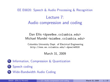
sults for a range of listeners which were generated in a National Institutes of Health (NIH) study of typical American hearingacuity. The quiet threshold is well approximated [46] by the non-linear function24 0.8(1)T ( f ) 3.64( f / 1000) 6.5e 0.6( f / 1000 3.3 ) 10 3 ( f / 1000 ) (dB SPL)qwhich is representative of a young listener with acute hearing. When applied to signal compression, Tq(f) could be interpreted naively as a maximum allowable energy level for coding distortions introduced in the frequency domain (Fig. 2). It isimportant to realize, however, that algorithm designers have no a priori knowledge regarding actual playback levels (SPL),and therefore the curve is often referenced to the coding system by equating the lowest point (i.e., near 4 kHz) to the energyin /- 1 bit of signal amplitude. In other words, it is assumed that the playback level (volume control) on a typical decoderwill be set such that the smallest possible output signal will be presented close to 0 dB SPL. This assumption is conservativefor quiet to moderate listening levels in uncontrolled open-air listening environments, and therefore this referencing practiceis commonly found in algorithms that utilize the absolute threshold of hearing. Psychoacoustic phenomena are typicallyquantified in terms of either dB SPL or dB sensation level (db SL). Therefore, perceptual coders must eventually referencethe internal PCM data to a physical scale such as SPL. A detailed example of this referencing is given in Section II.F.100Sound Pressure Level, SPL (dB)806040200210310Frequency (Hz)410Fig. 2. The absolute threshold of hearing in quiet. Across the audio spectrum, quantifies sound pressure level (SPL) required at each frequency such that an average listener will detect a pure tone stimulus in a noiseless environmentB. CRITICAL BANDSUsing the absolute threshold of hearing to shape the coding distortion spectrum represents the first step towards perceptual coding. Considered on its own, however, the absolute threshold is of limited value in the coding context. The detectionthreshold for quantization noise is a modified version of the absolute threshold, with its shape determined by the stimuli present at any given time. Since stimuli are in general time-varying, the detection threshold is also a time-varying function ofthe input signal. In order to estimate this threshold, we must first understand how the ear performs spectral analysis. A frequency-to-place transformation takes place in the cochlea (inner ear), along the basilar membrane. Distinct regions in thecochlea, each with a set of neural receptors, are “tuned” to different frequency bands. In fact, the cochlea can be viewed as abank of highly overlapping bandpass filters. The magnitude responses are asymmetric and non-linear (level-dependent).Moreover, the cochlear filter passbands are of non-uniform bandwidth, and the bandwidths increase with increasing frequency. The “critical bandwidth” is a function of frequency that quantifies the cochlear filter passbands. Empirical work byseveral observers led to the modern notion of critical bands [37][38][39][40]. We will consider two typical examples. Inone scenario, the loudness (perceived intensity) remains constant for a narrowband noise source presented at a constant SPLeven as the noise bandwidth is increased up to the critical bandwidth. For any increase beyond the critical bandwidth, theloudness then begins to increase. In this case, one can imagine that loudness remains constant as long as the noise energy ispresent within only one cochlear “channel” (critical bandwidth), and then that the loudness increases as soon as the noise energy is forced into adjacent cochlear “channels.” Critical bandwidth can also be viewed as the result of auditory detectionefficacy in terms of a signal-to-noise ratio (SNR) criterion. For example, the detection threshold for a narrowband noisesource presented between two masking tones remains constant as long as the frequency separation between the tones remainswithin a critical bandwidth (Fig 3a). Beyond this bandwidth, the threshold rapidly decreases (Fig 3c). From the SNR view4
Sound Pressure Level (dB)Sound Pressure Level (dB)point, one can imagine that as long as the masking tones are presented within the passband of the auditory filter (criticalbandwidth) that is tuned to the probe noise, the SNR presented to the auditory system remains constant, and hence the detection threshold does not change. As the tones spread further apart and transition into the filter stopband, however, the SNRpresented to the auditory system improves, and hence the detection task becomes easier, ultimately causing the detectionthreshold to decrease for the probe noise. f fFreq.Freq.fcb(b)Audibility Th.Audibility Th.(a) f ffcb(c)(d)Fig. 3. Critical Band Measurement Methods: (a,c) Detection threshold decreases as masking tonestransition from auditory filter passband into stopband, thus improving detection SNR. (b,d) Same interpretation with roles reversed252560002325500019Critical Bandwidth (Hz)Critical Band Rate, z (bark)212017151513111097540003000232000X CB filter center frequencies215191000X CB filter center frequencies31001731500010000 15000 2000005000 10000 15000 20000Frequency, f (Hz)00210579311 1310Frequency, f (Hz)15410(a)(b)Fig. 4. Two views of Critical Bandwidth: (a) Critical Band Rate, z(f), maps from Hertz to Barks, and(b) Critical Bandwidth, BWc(f) expresses critical bandwidth as a function of center frequency, in Hertz.The ‘Xs’ denote the center frequencies of the idealized critical band filter bank given in Table 1A notched-noise experiment with a similar interpretation can be constructed with masker and maskee roles reversed (Fig.3b,d). Critical bandwidth tends to remain constant (about 100 Hz) up to 500 Hz, and increases to approximately 20% of thecenter frequency above 500 Hz. For an average listener, critical bandwidth (Fig. 4b) is conveniently approximated [42] by[BWc ( f ) 25 75 1 1.4( f / 1000 )]2 0.69(Hz)(2)Although the function BWc is continuous, it is useful when building practical systems to treat the ear as a discrete set ofbandpass filters that conforms to Eq. (2). Table 1 gives an idealized filter bank that corresponds to the discrete points la-5
beled on the curve in Figs. 4a, 4b. A distance of 1 critical band is commonly referred to as “one bark” in the literature. Thefunction [42] f z ( f ) 13 arctan(.00076 f ) 3.5 arctan 7500 2 (Bark) (3)is often used to convert from frequency in Hertz to the bark scale (Fig 4a). Corresponding to the center frequencies of theTable 1 filter bank, the numbered points in Fig. 4a illustrate that the non-uniform Hertz spacing of the filter bank (Fig. 5) isactually uniform on a bark scale. Thus, one critical bandwidth comprises one bark. Intra-band and inter-band maskingproperties associated with the ear’s critical band mechanisms are routinely used by modern audio coders to shape the codingdistortion spectrum. These masking properties are described next.BandNo.123456789Center 500-1200012000-1550015500-Table 1. Idealized critical band filter bank (after[40]). Band edges and center frequencies for a collection of 25 rectangular critical bandwidth auditory filters that span the audio spectrumC. SIMULTANEOUS MASKING AND THE SPREAD OF MASKINGMasking refers to a process where one sound is rendered inaudible because of the presence of another sound. Simultaneous masking refers to a frequency-domain phenomenon that can be observed whenever two or more stimuli are simultaneously presented to the auditory system. Depending on the shape of the magnitude spectrum, the presence of certain spectralenergy will mask the presence of other spectral energy. Although arbitrary audio spectra may contain complex simultaneousmasking scenarios, for the purposes of shaping coding distortions it is convenient to distinguish between only two types ofsimultaneous masking, namely tone-masking-noise [40], and noise-masking-tone [41]. In the first case, a tone occurring atthe center of a critical band masks noise of any subcritical bandwidth or shape, provided the noise spectrum is below a predictable threshold directly related to the strength of the masking tone. The second masking type follows the same patternwith the roles of masker and maskee reversed. A simplified explanation of the mechanism underlying both masking phenomena is as follows. The presence of a strong noise or tone masker creates an excitation of sufficient strength on the basilar membrane at the critical band location to block effectively detection of a weaker signal. Inter-band masking has also beenobserved, i.e., a masker centered within one critical band has some predictable effect on1.210.80.60.40.200.20.40.60.811.2Frequency (Hz)1.41.61.824x 10F ig . 5 . I d e a liz e d c r itic a l b a n d f ilte r b a n k . I llu s tr a te s m a g n itu d e r e s p o n s e s f r o m T a b le 1d e te c tio n th r e s h o ld s in o th e r c r itic a l b a n d s . T h is e f f e c t, a ls o k n o w n a s th e s p r e a d o f m a s k in g , is o f te n m o d e le d in c o d in g a p p lic a tio n s b y a n a p p r o x im a te ly tr ia n g u la r s p r e a d in g f u n c tio n th a t h a s s lo p e s o f 2 5 a n d - 1 0 d B p e r b a r k . A c o n v e n ie n t a n a ly tic a l e x p r e s s io n [ 4 4 ] is g iv e n b y :SFdB ( x) 15.81 7.5( x 0.474) 17.5 1 ( x 0.474) 2 dB6(4)
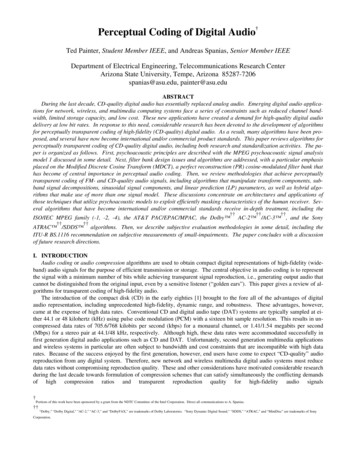
where x has units of barks and SFdb (x ) is expressed in dB. After critical band analysis is done and the spread of maskinghas been accounted for, masking thresholds in perceptual coders are often established by the [47] decibel (dB) relations:TH N ET - 14.5 - B(5)(6)TH T E N - Kwhere TH N and THT , respectively, are the noise and tone masking thresholds due to tone-masking-noise and noise-masking-SMRSNRMasking ToneMasking Thresh.Minimummasking Thresh.NMRSound Pressure Level (dB)tone, E N and ET are the critical band noise and tone masker energy levels, and B is the critical band number. Dependingupon the algorithm, the parameter K has typically been set between 3 and 5 dB. Of course, the thresholds of Eqs. 5 and 6capture only the contributions of individual tone-like or noise-like maskers. In the actual coding scenario, each frame typically contains a collection of both masker types. After they have been identified, these individual masking thresholds arecombined to form a global masking threshold. The global masking threshold comprises an estimate of the level at whichquantization noise becomes just-noticeable. Consequently, the global masking threshold is sometimes referred to as the levelof “Just Noticeable Distortion,” or “JND.” The standard practice in perceptual coding involves first classifying masking signals as either noise or tone, next computing appropriate thresholds, then using this information to shape the noise spectrumbeneath JND. Two illustrated examples are given in Sections II.E and II.F, which are on perceptual entropy, and ISO/IECMPEG Model 1, respectively. Note that the absolute threshold (Tq) of hearing is also considered when shaping the noisespectra, and that MAX(JND, Tq) is most often used as the permissible distortion threshold. Notions of critical bandwidth andsimultaneous masking in the audio coding context give rise to some convenient terminology illustrated in Fig. 6, where weconsider the case of a single masking tone occurring at the center of a critical band. All levels in the figure are given interms of dB SPL. A hypothetical masking tone occurs at some masking level. This generates an excitation along the basilarmembrane that is modeled by a spreading function and a corresponding masking threshold. For the band under consideration, the minimum masking threshold denotes the spreading function in-band minimum. Assuming the masker is quantizedusing an m-bit uniform scalar quantizer, noise might be introduced at the level m. Signal-to-mask ratio (SMR) and noise-tomask ratio (NMR) denote the log distances from the minimum masking threshold to the masker and noise levels, respectively.m-1mm 1Freq.Crit.BandNeighboringBandFig. 6. Schematic Representation of Simultaneous Masking (after [30])D. TEMPORAL MASKINGAs shown in Fig. 7, masking also occurs in the time-domain. For a masker of finite duration, non-simultaneous (temporal) masking occurs both prior to its onset as well as after its removal. In the case of audio signals, abrupt signal transients(e.g., the onset of a percussive musical instrument) create pre- and post- masking regions in time during which a listener willnot perceive signals beneath the elevated audibility thresholds produced by a masker. The skirts on both regions are schematically represented in Fig. 7. Essentially, absolute audibility thresholds for masked sounds are artificially increased priorto, during, and following the occurrence of a masking signal. Whereas premasking tends to last only about 5 ms, postmasking will extend anywhere from 50 to 300 ms, depending upon the strength and duration of the masker [42][48]. Temporalmasking has been used in several audio coding algorithms (e.g., [12][96][240][277]). Pre-masking in particular has been exploited in conjunction with adaptive block size transform coding to compensate for pre-echo distortions (section IV).7
Maskee AudibilityThreshold Increase 100150Time after
Department of Electrical Engineering, Telecommunications Research Center Arizona State University, Tempe, Arizona 85287-7206 . Audio coding or audio compression algorithms are used to obtain compact digital representations of high-fidelity (wide- . [101] for most for high-fidelity audio sources ( 88 kpbs given 44.1 kHz sampling). The lossy .