Transcription
c 2013 IEEE, Reprinted with permission, Georgiou G. and Voigt K., Self-Organizing Maps with a Single Neuron,Proceedings of International Joint Conference on Neural Networks, Dallas, Texas, USA, August 4-9, 2013, pp. 978–973.Self-Organizing Maps with a Single NeuronGeorge M. Georgiou and Kerstin VoigtGiven the 2-D nature of complex numbers, complex-valuedneurons will be used in the introduced self-organizing map.Complex-valued neural networks is an active area of research.[4]–[10]Abstract—Self-organization is explored with a single complexvalued quadratic neuron. The output is the complex plane. Avirtual grid is used to provide desired outputs for each input.Experiments have shown that training is fast. A quadraticneuron with the new training algorithm has been shown to haveclustering properties. Data that are in a cluster in the input spacetend to cluster on the complex plane. The speed of training andoperation allows for efficient high-dimensional data explorationand for real-time critical applications.II. C OMPLEX - VALUED NEURONSIt is desired that we have a 2-D output space so thatvisualization of the data in the output space is possible.Whereas two real neurons can be used to obtain the twocoordinates at the output, we chose to use a single complexneuron. This choice is motivated by the applicability to bothreal and complex data, and also, in the case of the quadraticneuron (below), by our ability to use results related to the fieldof values of the weight matrix. [11], [12] For example, if theinput vectors are normalized, the output is confined to the fieldof values, which is useful a priori information.I. I NTRODUCTIONELF-ORGANIZING maps have been extensively studiedand used in many applications. [1]–[3] In their basic form,they consist of an array of neurons which could be arrangedas a rectangular grid. During training each neuron is presentedwith each input vector X Rn in turn. There is a competitiveprocess during which a winner neuron c is found of which itsweight vector Mc Rn most closely matches X:Sc argmin(kX Mi k).A. The complex linear neuron(1)iThe complex linear neuron was introduced in [13] in thecontext of the LMS (Least-Mean Square) algorithm. The inputis X Cn and the weight vector of the neuron is W Cn .The output of the neuron is y W T X, the superscript (·)T isthe matrix (vector) transpose and y C is a complex scalar.The error is defined as εj dj yj , where dj C is thedesired valued for a given input vector Xj . The mean-squareerror isn1Xεj εj .(3)E 2 j 1The weights of the winner neuron c and those of the neuronswithin a neighborhood Nc on the neuron grid are modifiedaccording to this rule:(Mj (t) α(t)[X(t) Mj (t)] if j Nc (t)Mj (t 1) Mj (t)if j / Nc (t),(2)where t is the discrete time parameter, α is the learning rate,a small real value which decreases with time, and Nc is a setof neuron indices in the topological neighborhood around thewinning neuron with index c. The size of neighborhood Ncdecreases with time. After the learning process has iteratedthrough the input set of vectors many times, the neurons onthe grid are tuned to respond to different areas of the inputspace. In the normal operation, an input X is presented to theneurons on the grid and the winning neuron is identified asthe response. Vectors in close proximity in the input space willeither cause response from the same neuron or from a group ofneurons within close topological proximity to each other on thegrid. Thus, the two-dimensional grid provides a topologicallyconsistent map of the input space. Training usually takes manyiterations. The process is governed by many parameters, e.gthe initialization of weights, the schedule of decreasing of theneighborhood Nc , the size of the grid of neurons, and thedecreasing learning rate α(t). For example, a simple 2-D mapfrom the input space to a 2-D grid of neurons required 70, 000iterations.The gradient of the real function E with respect to W for aninput vector X, omitting the subscripts, is W E εX.(4)The overbar signifies complex conjugation. Hence, the onlinelearning rule that minimizes the mean-square error is thefollowing: W αεX.(5)The small real value α is the learning rate. The trainingof the neuron is done as in the real case: each input ispresented in turn, and the weight vector is adjusted accordingto Equation (5).B. The complex quadratic neuronThe real quadratic neuron has been briefly discussed [14].For input vector X Cn , the scalar complex output y X AX, where A Cn n , the weight matrix. The superscript(·) denotes the conjugate transpose. The output can be writtenGeorge M. Georgiou and Kerstin Voigt are with the School of ComputerScience and Engineering, California State University, San Bernardino, CA92407, USA (email: {georgiou, kvoigt}@csusb.edu).1
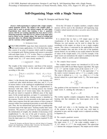
as a summation of the individual terms that involve thecomponents of X and A:y n XnXxj xk ajk .(6)j 1 k 1Using the same mean-square error as in Equation (3), thegradient of the error E with respect to weight ajk is ajk E εxj xk ,(7) A E εXX T .(8)or in vector format:The gradient descent learning rule that minimizes the meansquare error is A αεXX T ,(9)Fig. 1. The output of the grid data.where α, as always, is a small real value, the learning rate.The quadratic neuron has certain properties that other commonly used neurons, e.g. ones with sigmoid transfer functions,do not have. For example, the output can be scaled and rotatedby simply multiplying the weight matrix A by aeiθ , where a isthe scaling factor, a real scalar, and θ is the angle of rotation.If the input vectors are normalized, translation of the outputy by a complex scalar z can be achieved by replacing A withA zI:X (A zI)X X AX zX X y z.(10)These are desirable properties in cases where the neuron isalready trained and yet transformation of the output is needed.C. Mapping properties of the quadratic neuronTo explore the mapping properties of the quadratic neuron,a 2-dimensional data set arranged on a grid was generated. Therectangular data grid has diagonal points ( 1, 1) and (1, 1),and a total of 21 21 441 data points were generated.Each of the Figures 1, 2, 3 and 4, represents the outputof the quadratic neuron for same 2-dimensional data set.In each case, the weight matrix A was randomly assignedvalues. The figures show that the general structure of theinput data is preserved in the output. In the common case,the neurons on the grid in the Kohonen self-organizing mapsare randomly initialized, the structure of the input data needsto be discovered through training. The quadratic neuron startswith the advantage of having inherent topological properties.Fig. 2. The output of a grid data.Since the activation functions of both neurons are continuousfunctions of the input, proximity in the input space around asmall neighborhood of a point will be preserved in the output.When the quadratic neuron is used, there is experimentalevidence that clusters of data in the input space are preservedin the output space. This is the desired functionality of theintroduced new neural structure and algorithm.We begin the description of this new algorithm by defininga 2-D grid on the output space of the neuron, which is thecomplex plane. The grid, unlike the usual self-organizingmaps, is devoid of neurons. An example of such grid appearsin Figure 5. The intersection points of the grid serve as desiredvalues. For a given input vector X, the output y is computed.The desired output d to be used in the learning algorithm isdefined as the nearest intersection point of the grid lines. Inother words, the output snaps onto the nearest corner on thegrid. In practice, the snapping function snap can be definedin terms of a rounding function round, which rounds to thenearest integer and it can be found in many programminglanguages, such as Python. For example if one chooses a gridwith grid lines spaced at a distance 0.1 in both directions, theIII. T HE NEW SELF - ORGANIZING ALGORITHMInstead of having a grid of neurons where each is tunedto respond to an area of the input space, in the new selforganizing map we only have a single complex neuron. Thisneuron can be chosen to be either the linear one in Section II-Aor the quadratic one in Section II-B. The output is observedon the complex plane which provides a continuum in 2-Das opposed to the discrete grid of neurons in the usual selforganizing maps. This map can be used for data exploration,i.e. to visually gauge the structure of the input data which isnormally high dimensional and not amenable to visualization.2
where i 1, and the functions , return the real andthe imaginary parts of their argument, respectively. Since thegrid exists only implicitly through the snap function, it can becalled virtual grid. It can be limited to a specific rectangular,or square area. In that case, if the output y falls outside thegrid, the corresponding value d will be a point on the boundaryof the grid.After randomly initializing the weights of neuron, trainingproceeds as follows:1) Present input vector X to the neuron and compute theoutput y.2) Compute d snap(y), the nearest intersection of gridlines. This is the desired output for input X.3) Update the weights of the neuron using Equation (5) or(9), depending on which neuron is used.In each iteration, the above steps are carried out for each ofthe input vectors in the data set. The process is repeated fora number of iterations. Label information of the data is notused at any time. The learning rate could be decreasing withtime, as is the case with the Kohonen self-organizing maps,or there could be a maximum number of iterations, or therecould be a given minimum mean-square error over all inputsthat, when reached, stops the process. Normally the choicerests on experimentation and experience.The basic mechanism by which clustering is achieved withthe new algorithm could be explained as follows. A clusterin the input space will map to a similar region in the outputspace due to the continuity of the activation function. Otherdata vectors, not belonging to the cluster, may map to thesame region. Since the cluster data are more numerous, theywill cause the weights of the neuron to move so that theiroutputs remain close together in the same region of the grid.At the same time, the less numerous data will not have asmuch influence on the weights and will move away from thecluster in the output space.Fig. 3. The output of a grid data.Fig. 4. The output of a grid data.IV. R ESULTSA. The Iris data setClustering tests were conducted on the well known iris dataset. There are 150 4-dimensional (real) data vectors, whichbelong to three different classes. [15] In these experiments,the quadratic neuron was used with virtual grid lines spacedat 0.01. The grid onto which the output was allowed to snapwas limited to in the area of a square of size 2 centered at theorigin. A point outside the rectangle was snapping on a pointon the near boundary of the grid. For readability, grid linesin the figures are spaced at a larger distance. Run 1 and Run2 are representative of numerous runs, in which the generaltendency to clearly form the three clusters was observed.For both runs, the real and imaginary parts of the entries inthe weight matrix were initialized with random values in theinterval [ 0.01, 0.01]. The learning rate was set to α 0.001.The output for the data is color coded based on the class towhich it corresponds. For Run 1, the initial output is shown inFigure 6 and after 10 iterations through the data set in Figure 7.The corresponding figures for Run 2 are Figure 8 and 9.Fig. 5. The virtual grid on the output space.snap function can be defined as follows:d snap(y)round(10 (y))round(10 (y)) i1010round(10 (y)) round(10 (y)) (,),1010(11) 3
Fig. 6. Run 1: The initial distribution of the iris data.Fig. 8. Run 2: The initial distribution of the iris data.Fig. 7. Run 1: After 10 iterations the clusters are clearly formed.Fig. 9. Run 2: After 10 iterations the clusters are clearly formed.B. An artificial data setTo further test the algorithm, a data set was generated inR6 C6 that had two classes. Each class had 50 points(vectors). The classes were not overlapping, i.e. they werelinearly separable, and each was uniformly distributed in aunit sphere. Of interest in this experiment was the effect ofthe learning rate in the separation process of the two clustersand also the convergence of the algorithm. Figure 10 showsthe initial distribution of points of two classes at the outputof the quadratic neuron. As it can be seen in the figure,the two classes are initially thoroughly mixed together. Thenew self-organizing algorithm was applied as described in thethree experiments below In each case, a different learningrate α scheme was used. In these experiments, an infinitevirtual grid was used. In other words, the desired output wassimply the output of the snap(·) function; it was not limitedin a finite rectangular area. The virtual grid defined via thesnap(·) function had distance between grid lines, horizontaland vertical, 0.1. In all cases, the online version of the learningalgorithm was used as opposed to the batch method.Fig. 10. The initial distribution of the data.1) Learning rate α 0.01: When the learning rate α 0.01 was used, it was visually observed that the two classeswere already separated (linearly) at the output in about 45iterations through the data set. Continuing to run the algo4
rithm through 250 iterations, the two classes were movingaround, changing configurations. Their relative position wasonly slowly changing and the two classes remained separatedthrough the end of the process. Figure 11 shows the finalconfiguration of the points, after 250 iterations. We note thatthe points were spread out in a larger area, e.g. about 30 unitsin the y-direction, than likely they would have been if thegrid was limited, say, to the unit square around the origin.Figure 12 shows the error (Equation (3)) against the iterations.Fig. 12. The error fluctuates. However, after 45 iteration the two classesremained separatedFig. 11. The final distribution of the data.We see that there is continuous fluctuation, as opposed to theprototypical LMS error curve that monotonically decreaseswith the iterations, and the weight vector (matrix in thecurrent case) converges to a value. (Of course, instabilityis possible for the LMS algorithm, e.g. if the learning rateis large.) In this case, even though the weight matrix doesnot converge to a value and the points in the output movearound, if the algorithm were to stop at any point after 45iterations, the result would be acceptable. In general, withevery iteration, points change position, and hence there is apossibility, which increases with larger α, that their output willsnap on a different point on the virtual grid. This injects nonlinearity and non-monotonicity into the process, not unlikewhat happens in the Kohonen self-organizing maps when apoint, from one iteration to the next, causes another neuronto be the winner. Low error does not necessarily imply thatthe two classes are separated. It simply implies, that the pointsare nearer to their corresponding desired outputs on the virtualgrid.2) Learning rate α 0.001: When the learning rate wasα 0.001, it proved to be very small, and there was very littlemovement of points in the output. The initial distribution ofpoints in output (Figure 10) remained almost identical to thefinal one, after 250 iterations (not shown). Figure 13 showsthe plot of the error against the iterations. Even though theerror decreases, the configuration of the points does not changein any substantial way from the initial output, before anyiterations of the algorithm.Fig. 13. Although the error decreases, the configuration of the pointsin the output essentially remains the same as the initial one.3) Decaying learning rate: The learning rate α was initially0.01 and then was decreased according to this formula:αn 0.01 e n(n 3)k,(12)where n is the iteration and k is constant. This formula and theconstant k 10, 000 were found by experimentation: if thedecay was too fast, the clusters did not have the opportunityto form, and the points settled in a fixed position. If the decaywas too slow, the weights were changing and the points weremoving around. The ideal decay would be for the clustersto have the opportunity to separate, and then become fixedin position. Figure 14 shows the error initially erraticallyfluctuating, and after about 150 iterations it becomes smoother.The two clusters settled in essentially the final configuration(iteration 250) from iteration 100. (Figure 15)C. The linear neuronIn experiments with the linear neuron using the iris data,similar clustering behavior was observed. It was observed that5
V. C ONCLUSIONBy introducing the concept of the virtual grid, where inputvectors define their own desired outputs, self-organizationhas been shown to be possible with a single complex neuron.The same algorithm can be easily modified using tworeal neurons. Evenly distributed data on a 2-D array did notcause clustering behavior in the output. The new fast andeconomical method, involving only one neuron, promises tobe useful in the exploration of high-dimensional data, and inapplications where self-organizing maps are typically used.It will be particularly suitable for real-time and other timecritical applications. Given that training with the virtual gridis a local technique, one may speculate whether analogousself-organizing mechanisms exist in biological systems.VI. B IBLIOGRAPHYFig. 14. The error with decaying learning rate.R EFERENCES[1] T. Kohonen, “Self-organized formation of topologically correct featuremaps,” Biological Cybernetics, vol. 43, 1982, reprinted in [16].[2] ——, Self-Organization and Associative Memory, 3rd ed.Berlin:Springer-Verlag, 1989.[3] ——, “The self-organising map,” Proceedings of the IEEE, vol. 78,no. 9, pp. 1464–1480, 1990.[4] A. Hirose, Ed., Complex-Valued Neural Networks: Theories and Applications. World Scientific Publishing, 2003.[5] A. Hirose, Complex-Valued Neural Networks, ser. Studies in Computational Intelligence. Springer, 2006, vol. 32.[6] ——, Complex-valued Neural networks.Saiensu-sha, 2005, inJapanese.[7] T. Nitta, Complex-valued Neural Networks: Utilizing High-dimensionalParameters, 1st ed. Information Science Reference, 1 2009.[8] I. N. Aizenberg, Complex-Valued Neural Networks with Multi-ValuedNeurons, ser. Studies in Computational Intelligence. Springer, 2011,vol. 353.[9] S. Suresh, N. Sundararajan, and R. Savitha, Supervised Learning withComplex-valued Neural Networks, ser. Studies in Computational Intelligence. Springer, 2013, vol. 421.[10] Z. Chen, S. Haykin, J. J. Eggermont, and S. Becker, CorrelativeLearning: A Basis for Brain and Adaptive Systems (Adaptive andLearning Systems for Signal Processing, Communications and ControlSeries), 1st ed. Wiley-Interscience, 10 2007.[11] K. E. Gustafson and D. K. Rao, Numerical Range: The Field of Valuesof Linear Operators and Matrices (Universitext), 1st ed. Springer, 111996.[12] R. A. Horn and C. R. Johnson, Topics in Matrix Analysis. CambridgeUniversity Press, 5 1991.[13] B. Widrow, J. McCool, and M. Ball, “The complex lms algorithm,”Proceedings of the IEEE, vol. 63, no. 4, pp. 719–720, 1975.[14] G. Georgiou, “Exact interpolation and learning in quadratic neuralnetworks,” in IJCNN ’06. International Joint Conference on NeuralNetworks, 2006, pp. 230–234.[15] R. A. Fisher, “The use of multiple measurements in taxonomic problems,” Annals of Eugenics, vol. 7, no. II, pp. 179–188, 1936.[16] J. Anderson and E. Rosenfeld, Eds., Neurocomputing: Foundations ofResearch. Cambridge: MIT Press, 1988.Fig. 15. The final configuration of the clusters with decaying learningrate.on many occasions, in the initial output a class was alreadyseparable from the other two classes. Nevertheless, applyingthe algorithm showed that in general there is a tendency forthe formed clusters to remain intact. More experiments areneeded to compare the linear neuron with the quadratic one.6
and for real-time critical applications. I. INTRODUCTION S ELF-ORGANIZING maps have been extensively studied and used in many applications. [1]–[3] In their basic form, they consist of an array of neurons which could be arranged as a rectangular grid. During training each neuron is pre