Transcription
Discovering Plate BoundariesTeachers Guide 2: A Tour of the MapsDiscovering Plate BoundariesTeachers Guide: Part 2“A Tour of the Maps”Dale S. SawyerProfessor of Earth ScienceRice UniversityHouston, Texasdale@rice.eduHi, my name is Dale Sawyer. I am a Professor of Earth Science at Rice University in Houston Texas.I have worked with colleagues to develop a classroom exercise called Discovering Plate Boundaries,intended to lead students to discover for themselves the types of tectonic plate boundaries. Afterdoing the exercise, they should be able to relate geological observations at plate boundaries to theimportant physical processes that occur there. This presentation is one part of the Teachers Guide Ihave put together to help the classroom teacher prepare to use the exercise. I hope that you find ituseful. I welcome comments about the exercise and how it can be improved via my email addressdale@rice.edu .Lets begin!Dale S. SawyerRice University1
Discovering Plate BoundariesTeachers Guide 2: A Tour of the MapsThe key resource that your students will use in this exercise are four data maps. In this presentation I hope to:1. introduce the data used in each map,2. tell you where I got the data,3. show you how the data are displayed,4. show you some key parts of the data, and what your students can/should see as theycomplete the exercise.The data maps used in Discovering Plate Boundaries are, a map of seafloor age, a map showing earthquakelocation and depth, a map showing locations of recent volcanic activity, and a map showing the Earth’stopography and bathymetry.Dale S. SawyerRice University2
Discovering Plate BoundariesTeachers Guide 2: A Tour of the MapsThis slide contains details about the map projection. IT MAY BE SKIPPED.The projection for all the maps in Discovering Plate Boundaries is Mercator. We chose this because it is the mostcommonly used projection for world maps, and your students have undoubtedly seen maps of this sort before.Other positive characteristics of Mercator maps are that north is up and east is horizontal to the right everywhereon the map, and that the graticule is rectangular so that it is easy to read latitude and longitude from the map.Less desirable characteristics are that shape and area are distorted at high latitudes (far north and south of theequator), and that the North and South poles cannot be represented because they would plot infinitely far from theequator.You will notice that the area of a continent at high latitude, for example Greenland, is exaggerated with respectto that of a continent near the equator, such as Africa. Africa is actually much larger than Greenland! Also notethat Antarctica appears huge and occupies the entire bottom edge of the map.The graticule of a map is the grid of latitude and longitude lines displayed over the map. For these maps, thegraticule is spaced at 30 degrees in both latitude and longitude. The lines of constant latitude run east/west andare called “parallels.” The lines of constant longitude run north/south and are called “meridians.”The maps cover the area between 80 degrees South latitude and 80 degrees North latitude. The maps are centeredon longitude 0 degrees,which is the Prime Meridian that passes through Greenwich, England. This is of course anarbitrary choice. Most students in the US have most often seen world maps centered on the US! When I was ateenager, I visited an Australian school and thought the world map at the front of the classroom looked verypeculiar. After a bit of thought, I realized that it was because the map was centered on Australia and the mapedges were in the Atlantic Ocean!The coastlines are an important reference point for students. This is how they can recognize geographic locations.The coastline data for these maps include the land/ocean boundaries and the boundaries of all lakes larger than5000 sq. km.Dale S. SawyerRice University3
Discovering Plate BoundariesTeachers Guide 2: A Tour of the MapsThis map shows the plate boundaries that are used in the Discovering Plate Boundaries exercise. These data wereobtained from Dietmar Muller, a scientist at the University of Sydney in Australia.While most plate boundary locations are generally agreed upon by scientists, some are not. Other plate boundarymaps may be expected to deviate from this one in certain details. Neither is necessarily right or wrong. To get atthe differences, one must dig deeper into the observations and interpretations than is appropriate for this type ofclassroom exercise. Therefore, when students point out discrepencies, I praise them for their observation skillsbut try to lead them away from concluding that this makes the entire exercise suspect! That is simply not the case.Dale S. SawyerRice University4
Discovering Plate BoundariesTeachers Guide 2: A Tour of the MapsThis is a small version of the map for the scientific specialty of “Volcanology.” Each red dot on this maprepresents some type of volcanic activity active within the last 10,000 years. Most of the dots representvolcanoes, while others represent hot springs, geysers, and other volcanic/thermal features. The data wereassembled and may be obtained freely from the Smithsonian Institution in Washington, DC, USA.Dale S. SawyerRice University5
Discovering Plate BoundariesTeachers Guide 2: A Tour of the MapsI have added the plate boundary lines (in gray) to the volcanic activity map. I will use close-up views of thisversion of the map to describe how volcanic features relate to plate boundaries and plate boundary processes. Inthis presentation, I will be emphasizing the observations that students can make. In a second presentation, I willdiscuss the plate boundary processes and the meaning of the observations.You may want to use this slide in presentations to your class.Dale S. SawyerRice University6
Discovering Plate BoundariesTeachers Guide 2: A Tour of the MapsLines of volcanic activity are generally associated with convergent (subducting) plate boundaries. In thesecases, the line of volcanoes is located roughly parallel to the plate boundary and generally forms a tight line. Thevolcanoes are located on the “over-riding” plate of the subducting plate boundary.If the convergent (subducting) plate boundary is between two oceanic plates, the boundary usually has an arcuateshape. The line of volcanoes usually form a chain of islands that we call a volcanic arc. The arc is usually convexin the direction of the downgoing plate and concave in the direction of the over-riding plate.In this perfect example of the pattern, the volcanos shown by the arrow in this figure form the Aleutian IslandChain. The volcanoes are located in a tight line to the north of the plate boundary. The North American Plate(which includes Alaska and the Bering Sea) is the over-riding plate. The Pacific Plate is the down-going plate atthis subduction system.Dale S. SawyerRice University7
Discovering Plate BoundariesTeachers Guide 2: A Tour of the MapsNote that this kind of map wraps around at its edge!Right side of mapLeft side of mapYou may want to ask your students to note that features on the Earth sometimes cross from one side of the map tothe other. The arrow pairs in this slide show that the Aleutian Island Arc and the landmass of Siberia extendacross the map edges.This would not be a problem if we were doing all our work with a globe. It is a problem when we work with flatmaps.Dale S. SawyerRice University8
Discovering Plate BoundariesTeachers Guide 2: A Tour of the MapsThe Indonesian volcanic arc marked with the arrow is another fine example of a Convergent (subducting) plateboundary between two oceanic plates. It has the same characteristics as the Aleutian example. As you can see,this is a very complicated part of the world (in a plate tectonic sense!).Dale S. SawyerRice University9
Discovering Plate BoundariesTeachers Guide 2: A Tour of the MapsNorth American PlateEurasian PlatePacific PlateJapan, marked with the arrow, is part of a complex set of shorter subducting plate boundary segments. Note thateach has the key properties I mentioned: arcuate shape and volcanoes in a tight line roughly parallel to the plateboundary. Which plate is the down-going plate in this system? Which plate is the over-riding plate in thissystem?I hope you said that the Pacific Plate is going down beneath the Eurasian and North American Plates!Dale S. SawyerRice University10
Discovering Plate BoundariesTeachers Guide 2: A Tour of the MapsNazca PlateSouth American PlateAntarctic PlateThis is an example of a Convergent (subducting) plate boundary in which oceanic crust (Nazca and AntarcticPlates) is being subducted beneath continental crust (South American Plate). Note that at such a boundary, it willalways be the oceanic plate as the down-going plate and the continental plate as the over-riding plate. This isbecause oceanic crust is almost always denser than continental crust.Note that the main differences between this plate boundary and the boundaries we saw in the Aleutian and thewestern Pacific are that the volcanoes here are part of a high mountain system (the Andes Mountains) rather thanan island chain, and that the arcuate shapes are often not as obviously developed. The other patterns hold, withthe volcanoes in a tight line, parallel to the plate boundary, and on the over-riding plate.Note that in the lower right hand corner of this map is a short, well developed, volcanic arc related to thewestward subduction of the South American Plate under the Antarctic Plate. We call this the Scotian Arc.Dale S. SawyerRice University11
Discovering Plate BoundariesTeachers Guide 2: A Tour of the MapsYour students are likely to observe this line of volcanoes and ask why it does not lie along a plate boundary. Theanswer is that it does lie along a plate boundary, but the south end of that boundary is ill defined and poorlyunderstood! I have therefore elected to leave that boundary out of the plate boundaries included in the exercise.The students should be aplauded for their skills of observation and pattern recognition!Dale S. SawyerRice University12
Discovering Plate BoundariesTeachers Guide 2: A Tour of the MapsEurasian PlateIndian PlateThe final type of Convergent plate boundary is at the collision of two continents. In this example, the Indian plateis colliding with the Eurasian plate. As we see here, there is often no volcanic activity associated with this type ofplate boundary.Dale S. SawyerRice University13
Discovering Plate BoundariesTeachers Guide 2: A Tour of the MapsLooking at this map, your students should observe that Divergent plate boundaries are only sporadicallyassociated with volcanoes. Along the Mid Atlantic Ridge, shown in the slide, then only volcanism appears inIceland (marked with the arrow near the top of the slide) and the Canary Islands (marked with the arrow in thelower part of the slide).This is due to the type of dataset the Smithsonian Institution has assembled. They have chosen to show onlyvolcanic features that can be observed on land surfaces. This means that this map only shows a dot where avolcano has grown to produce an island or has erupted on a continent. We now know that by far most of thevolcanism on Earth actually happens under the ocean along mid-ocean ridges, but these volcanoes are typicallynot observed, are underwater, and don’t make it to the Smithsonian list. I discuss this with students as a greatexample that when doing real science, the perfect dataset for answering your question usually does not exist. Thedata are usually lacking in some way; they may be incomplete, they may contain errors, they may even bemisleading. Real science happens in spite of that, because the human brain is able to recognize patterns in lessthan perfect data!Dale S. SawyerRice University14
Discovering Plate BoundariesTeachers Guide 2: A Tour of the MapsTransform plate boundaries, like the plate boundary along the coast of California, may be associated with a broadzone of volcanic activity or may have none. The part of this plate boundary next to the orange bar is a transformplate boundary. The part of this plate boundary next to the green bar is a convergent (subducting) plate boundary.Note that the line of vocanoes becomes tighter where subduction is occurring. This is the Cascade Range inOregon and Washington, made of of well known volcanoes such as Mt. Ranier and Mt. St. Helens.Dale S. SawyerRice University15
Discovering Plate BoundariesTeachers Guide 2: A Tour of the MapsThis is a small version of the map for the scientific specialty of “Seismology.” Each dot on this map representsthe “epicenter” of an earthquake. The epicenter of an earthquake is the surface location directly over the“hypocenter” of the earthquake. The hypocenter is the location of the break in the rocks, whose relativemovement caused the earthquake.The color of the dots represents the depth of the hypocenter of the earthquake. Red dots are earthquakes between0 and 33 km depth. Yellow dots are earthquakes between 33 and 70 km depth. Green dots are earthquakesbetween 70 and 300 km depth. Blue dots are earthquakes between 300 and 700 km depth. Note that in manyplaces, dense patterns of dots may cover other colors of dots. The red dots are plotted first, followed by yellow,green, and then blue.You may be surprised that we have not shown earthquake magnitude on this map. While there is someassociation with the size of the largest earthquakes and plate boundary types, the depth distribution is actuallymuch more informative.These data were obtained from Incorporated Research Institutions for Seismology (IRIS). They includeearthquakes that occurred between 1990 and 1996. Any recent 6 year period could be used to construct a similarmap. This interval was chosen in 1997 when I created “Discovering Plate Boundaries.”Dale S. SawyerRice University16
Discovering Plate BoundariesTeachers Guide 2: A Tour of the MapsThis is the same earthquake location and depth map with the plate boundaries added in gray. I use closeups ofthis map in the detailed descriptions which follow.You may want to use this slide in presentations to your class.Dale S. SawyerRice University17
Discovering Plate BoundariesTeachers Guide 2: A Tour of the MapsDivergent plate boundaries show up very clearly in the earthquake data. The arrow points to the Mid-AtlanticRidge. The earthquakes along mid-ocean ridges are dominantly shallow, less than 33 km and shown as red dots.They occur on the plate boundary, not offset to one side or the other. You cannot really tell from these maps, butthe earthquake activity is generally confined to a boundary region about 10 km wide. They occur on both theplate boundary segments that are perpendicular to the spreading direction and the segments that are parallel to thespreading direction. The spreading direction here is roughly east - west. The roughly north/south segments of theplate boundary are actually the “spreading center” segments and are divergent plate boundary segments. Theroughly east-west segments of the plate boundary are the “transform fault” segments and are transform plateboundary segments.The earthquakes along mid-ocean ridges are generally small, with Richter magnitudes less than about 6.0.Dale S. SawyerRice University18
Discovering Plate BoundariesTeachers Guide 2: A Tour of the MapsConvergent (subducting) plate boundaries are also seen quite easily in the earthquake map. Subducting plateboundaries are characterized by shallow earthquakes occurring on both sides of the plate boundary andintermediate and deep earthquakes occurring on one side of the boundary. The deper quakes occur on the overriding plate side of the boundary. The quakes of different depths tend to form bands at increasing depth atincreasing distances from the plate boundary. You can see this pattern in the Aleutian Island Arc part of the plateboundary between the pacific plate and the North American plate. The deepest quakes on this margin are shownin green, telling us that they lie between 70 and 300 km depth. Shortly, we will see subducting plate boundariesthat include even deeper earthquakes. Note that in this area. The red band straddles the plate boundary, the yellowband is displaced to the north, and the green band is displaced farther north. These earthquakes form theWaddati-Beniof zone and lie near the boundary between the top of the down-going plate and the over-ridingplate.Dale S. SawyerRice University19
Discovering Plate BoundariesTeachers Guide 2: A Tour of the MapsThe deepest Waddati-Beniof zone is associated with the Tonga Trench seen in this slide. It is cut by the mapboundary, and thus takes a bit more effort to put it together. As in the Aleutian example, the red band ofearthquakes straddles/covers the plate boundary, The yellow, green, and blue bands follow sequentially to thewest. Here the Australian plate is over-riding the Pacific plate. The colored bands are closely spaced in thisexample because the Pacific plate is plunging steeply under the Australian plate. Where the subducting plate isgoing down at a less steep angle, the bands are more spaced out.Dale S. SawyerRice University20
Discovering Plate BoundariesTeachers Guide 2: A Tour of the MapsThe Western Pacific Ocean has a number of convergent (subducting) plate boundaries that stand-out in theearthquake map. Note the variations in the depth of the deepest earthquakes in the different subduction systems.All include green band depths (up to 300 km), but only some include blue bands representing quakes deeper than300 km. Note also that the spacing of the bands varies, showing different angles of descent for the downgoingplates. The arcuate shape of these plate boundaries also shows up very clearly.Dale S. SawyerRice University21
Discovering Plate BoundariesTeachers Guide 2: A Tour of the MapsThis slide shows one more example of a subducting plate boundary involving two oceanic crust plates, and twoexamples of oceanic crust of the down-going plate being subducted under continental crust on the over-ridingplate. I am confident that you can pick put which is which! Note that the earthquake depth pattern we associatewith subduction is still present. The colored bands for earthquakes under South America are widely spaced. Thisis an example of a very shallowly dipping subducting plate. It is shallow here because the oceanic crust of thispart of the Pacific plate is very young and therefore relatively buoyant. The subduction zone under CentralAmerica is much steeper, but does not penetrate as deeply as the South American subduction system.Dale S. SawyerRice University22
Discovering Plate BoundariesTeachers Guide 2: A Tour of the MapsTransform plate boundaries are typically the site of many shallow earthquakes along a sometimes diffuse zone.The plate boundary between the Pacific plate and the North American plate in California is a good example.Although sometimes very damaging because of big cities in this area, the largest earthquakes on transformboundaries are usually not as large as the largest subduction zone earthqaukes.Dale S. SawyerRice University23
Discovering Plate BoundariesTeachers Guide 2: A Tour of the MapsHimalaya MountainsConvergent (continental collision) plate boundaries are usually marked by very diffuse zones of earthquakes thatare mostly shallow, but sometimes intermediate in depth. The Indian plate is colliding with the Eurasian plate,forming the Himalayan Mountains. The effects of this collision are also felt as earthquakes in much of China.Dale S. SawyerRice University24
Discovering Plate BoundariesTeachers Guide 2: A Tour of the MapsEarthquake activity is particularly concentrated in the Medditeranean are in this map. The area is characterizedby a complicated pattern of small tectonic plates that are continually rubbing against one another. This producesthe many bands of earthquakes that you can see on the map. The quakes are almost all shallow. The main eastwest difuse band of earthquakes is related to a general convergence between the African plate and the Eurasianplate. The seismicity appears denser in this area that any other (except perhaps California) because there aremany seismograph stations nearby. This means the the earthquake catalog includes many earthquakes smallerthan would be observed in other parts of the world. This is a good example to discuss with your students.Datasets often have uneven coverage, and it is important that the scientist be aware of this when interpreting theirdata!Dale S. SawyerRice University25
Discovering Plate BoundariesTeachers Guide 2: A Tour of the MapsThis is a small version of the map for the scientific specialty of “Geochronology.” The colors represent the age ofthe oceanic crust. There is a color bar on the right side of the map that shows the ages in millions of years. At thebottom of the scale, red represents very young oceanic crust, formed less than 9.7 million years ago. The oldestoceanic crust is represented in blue, and is between 154 and 180 million years old. Data are only shown for areasof the plates that consist of oceanic crust and for which the age is well determined. No data are shown for theland areas because they are underlain by continental crust. No data are shown for some continental margin areasbecause the sediment cover is great and it is not currently possible to determine the age of oceanic crust there. Nodata are shown is some high latitude areas because there are not yet sufficient data coverage to reliably determineages there.Note that all oceanic crust on Earth is younger than about 180 million years. This is actually surprising given thatthe Earth was formed about 4,600 million years ago and there are areas of the continents where the rocks areknown to be almost 4,000 million years old. The oceans are young because old ocean crust becomes quite denseand tends to be subducted back into the mantle. Thus it does not hang around on the surface of the Earth verylong. Continental crust is relatively quite light, both when it is young and when it is old, so it tends to stay at thesurface nearly forever.These data were obtained from Dietmar Muller, a scientist at the University of Sydney in Australia.Dale S. SawyerRice University26
Discovering Plate BoundariesTeachers Guide 2: A Tour of the MapsAs you have seen before, this is a version of the map with plate boundaries superimposed in gray, and I will bereferring to close-ups of this map.You may want to use this slide in presentations to your class.Dale S. SawyerRice University27
Discovering Plate BoundariesTeachers Guide 2: A Tour of the MapsMid Ocean Ridges, the main type of Divergent plate boundary, practically jump off the map at you! At an activemid-ocean ridge, new oceanic crust is being generated, so the plate boundary should always lie along a band ofred on the map. The newly generated crust is formed at the ridge and then moves symmetrically away from theridge in both directions. Thus the crust becomes older as you move away from a mid-ocean ridge. This pattern iseasily seen for the Mid Atlantic ridge in the slide.The oldest oceanic crust in the Atlantic Ocean is found on the margins of North America and Africa. The bluecrust there was formed when Africa had just started to spread away from North America.Dale S. SawyerRice University28
Discovering Plate BoundariesTeachers Guide 2: A Tour of the MapsThis is the Mid-Atlantic Ridge in the far North Atlantic Ocean. The divergent plate boundary goes right throughIceland. There you can observe volcanism and seafloor spreading happening at the surface.Before going forward to the next slide, please notice how wide the red, orange, and yellow bands are in thisimage. This is an example of a “slow-spreading” ridge. New crust is created at this ridge at a rate of about 4 cmper year. In the next figure we will look at a ridge spreading about 3 times as fast! Do you expect the red, orange,and yellow bands to be wider or narrower in that image?While you are thinking, I would also like to point out a mid-ocean ridge that was active in the past but is notactive now. It is in the Labrador Sea, between Canada and Greenland. It has a seafloor age pattern like that of anactive ridge except that the band in the middle is not red. That means it stopped spreading at “orange time.” Thatwas between 33.1 and 40.1 million years ago (check 2 slides back for the legend which gives the ages of eachcolor band). That is why there is no plate boundary between Canada and Greenland. They are both part of theNorth American plate now.Dale S. SawyerRice University29
Discovering Plate BoundariesTeachers Guide 2: A Tour of the MapsThe arrow points to the East Pacific Rise. It is also a divergent plate boundary. It is displayed at the same scale asthe last slide. Are the red, orange, and yellow bands on either side of the spreading center wider? They sure are!This is the fastest spreading rate ridge; it is creating about 12 cm of new oceanic crust on each side of the ridgeeach year. That is about as fast as your hair grows; fast huh?There are two spreading center ridges that branch from the East Pacific Rise and go to the east. They arespreading more slowly. The two small enclosed circles in the lower middle of the slide are microplates. They arebordered by divergent and transform plate boundaries on all sides.Dale S. SawyerRice University30
Discovering Plate BoundariesTeachers Guide 2: A Tour of the MapsThis is the Indian Ocean. It has a network of divergent plate boundaries. Note the variations in spreading rate.Also note that fast spreading ridges have fewer but larger transform offsets than slow spreading ridges. Here thecontrast is greatest between the ridge in the lower right and the lower left of the slide.Now, a puzzler for you! Can you find two extinct spreading centers in this slide? Can you tell which of the twobecame extinct first?Dale S. SawyerRice University31
Discovering Plate BoundariesTeachers Guide 2: A Tour of the MapsThe two black dotted lines show extinct spreading centers. The extinct spreading center in the upper left, stoppedspreading long ago (in green time). The spreading center in the upper right stopped spreading in yellow to orangetime, much more recently. We can use the colorbar from the map to attach numerical ages to the time duringwhich these spreading centers were active. This is not actually part of the exercise,but it is an example of theamazing amount of information contained in these data!Dale S. SawyerRice University32
Discovering Plate BoundariesTeachers Guide 2: A Tour of the MapsConvergent (subducting) plate boundaries have no consistent seafloor age along the boundary. We see here thatalong the subducting boundary on the west side of South America, the age of the oceanic crust being subductedvaries from pale orange to red age. This is because oceanic crust of any age can be subducted. This is asubduction system with continental crust in the over-riding plate. Because it is continental there are no seafloorage data. Frequently the students will describe such boundary as one between data and no data. For olderstudents I usually push on them to think about that a bit deeper and describe the boundary in terms of the age ofwhat is being subducted rather than just the presence or absence of data.Dale S. SawyerRice University33
Discovering Plate BoundariesTeachers Guide 2: A Tour of the MapsThe Western Pacific is complicated. The students should note that in the few places where there are data near thesubducting boundaries, the age of the oceanic crust is varying. Putting this whole story together will likely onlycome in the second phase of the exercise when the students put different kinds of data together for this area.As a side note, the oldest oceanic crust known is in the blue area of this slide. Because it is so close to thesubduction boundaries of the western Pacific, we know that it won’t be but a few million years before it issubducted and recycled into the mantle.Do you see any extinct spreading centers here? There is one in the lower left that stopped spreading at orangetime and one in the center that stopped spreading later in orange time!Dale S. SawyerRice University34
Discovering Plate BoundariesTeachers Guide 2: A Tour of the MapsHere we see the age pattern in oceanic crust off the subduction boundary of the Aleutians and the transformboundary along the California coast. Transform plate boundaries are like subduction boundaries in that the agecan vary along the boundary.Dale S. SawyerRice University35
Discovering Plate BoundariesTeachers Guide 2: A Tour of the MapsThis is a small version of the map for the scientific specialty of “Geography.” The colors represent the elevationof the land surface and of the bottom of the ocean. Elevation is expressed in the color bar in meters. The pale bluethrough dark blue and then purple colors are shallow to deep ocean areas. The dark green through brown, gray,and white are low to high land elevations.These data were obtained from the US National Geophysical Data Center and are called the “ETOPO5” dataset.ETOPO5 stands for Earth Topography at 5 minute spacing.Dale S. SawyerRice University36
Discovering Plate BoundariesTeachers Guide 2: A Tour of the MapsThis is a version of the map with plate boundaries superimposed as narrow red lines, and I will be referring toclose-ups of this map.You may want to use this slide in presentations to your class.Dale S. SawyerRice University37
Discovering Plate BoundariesTeachers Guide 2: A Tour of the MapsWe will start with the topographic signature of divergent plate boundaries. The first observation is that thedivergent boundary follows the peak of a seafloor mountain range. The water depth is greater on each side of theplate boundary. The depth change is
The projection for all the maps in Discovering Plate Boundaries is Mercator. We chose this because it is the most commonly used projection for world maps, and your students have undoubtedly seen maps of this sort before. Other positive characteristics of Mercator maps are that north is up and ea