Transcription
JSSJournal of Statistical SoftwareOctober 2007, Volume 21, Issue 5.http://www.jstatsoft.org/Self- and Super-organizing Maps in R: The kohonenPackageRon WehrensLutgarde M. C. BuydensRadboud University NijmegenRadboud University NijmegenAbstractIn this age of ever-increasing data set sizes, especially in the natural sciences, visualisation becomes more and more important. Self-organizing maps have many featuresthat make them attractive in this respect: they do not rely on distributional assumptions,can handle huge data sets with ease, and have shown their worth in a large number ofapplications. In this paper, we highlight the kohonen package for R, which implementsself-organizing maps as well as some extensions for supervised pattern recognition anddata fusion.Keywords: self-organizing maps, visualisation, classification, clustering.1. IntroductionDue to advancements in computer hardware and software, as well as in measurement instrumentation, researchers in many scientific fields are able to collect and analyze datasets ofsteadily increasing size and dimensionality. Exploratory analysis, where visualization plays avery important role, has become more and more difficult given the increasing dimensionalityof the data. There is a real need for methods that provide meaningful mappings into twodimensions, so that we can fully utilize the pattern recognition capabilities of our own brains.There are many approaches to mapping a high dimensional data set into two dimensions, ofwhich principal component analyis (PCA, Jackson 1991) is probably the most used. However,in many cases more than two dimensions are needed to provide a reasonably useful picture ofthe data so that visualisation remains a problem. Moreover, PCA in its pure form does notincorporate information on how objects should be compared; the standard Euclidean distancemeasure is not always the optimal dissimilarity measure. Methods starting from distance orsimilarity matrices, in this respect, may prove more useful. First of all, such methods scalewell to large numbers of variables, and second, by choosing an appropriate distance function
2kohonen: Self- and Super-organizing Maps in Rfor the data at hand, one concentrates on those aspects of the data that are most informative.One approach to the visualization of a distance matrix in two dimensions is multi-dimensionalscaling (MDS) and its many variants (Cox and Cox 2001). This technique aims to find aconfiguration in two-dimensional space whose distance matrix in some sense approaches theoriginal distance matrix, calculated from the high-dimensional data. The procedure may endup in a local optimum and may have to be performed several times, which for larger numbersof objects can be quite tedious. Moreover, there is no simple way to project new objects intothe same space.Self-organizing maps (SOMs, Kohonen 2001) tackle the problem in a way similar to MDS, butinstead of trying to reproduce distances they aim at reproducing topology, or in other words,they try to keep the same neighbours. So if two high-dimensional objects are very similar, thentheir position in a two-dimensional plane should be very similar as well. Rather than mappingobjects in a continuous space, SOMs use a regular grid of “units” onto which objects aremapped. The differences with MDS can be seen as both strengths and weaknesses: where ina 2D MDS plot a distance – also a large distance – can be directly interpreted as an “estimate”of the true distance, in a SOM plot this is not the case: one can only say that objects mappedto the same, or neighbouring, units are very similar. In other words, SOMs concentrate onthe largest similarities, whereas MDS concentrates on the largest dissimilarities. Which ofthese is more useful depends on the application.SOMs have seen many diverse applications in a broad range of fields, such as medicine, biology, chemistry, image analysis, speech recognition, engineering, computer science and manymore; a bibliography of more than 7,700 papers is available at the website of the universitywhere Teuvo Kohonen initiated the SOM research (Helsinki University of Technology – CISLaboratory 2007). From the same research group one can obtain C source code for SOMsand a MATLAB-based package (Helsinki University of Technology – CIS Laboratory 2006).For R (R Development Core Team 2007), two packages are available from the ComprehensiveR Archive Network (CRAN, http://CRAN.R-project.org/) implementing standard SOMs:the som package, by (Yan 2004), and the class package, part of the VR package bundle(Venables and Ripley 2002).The latter provided the basis for the kohonen package, described in this paper and alsoavailable from CRAN. The kohonen package features standard SOMs and two extensionsthat make it possible to use SOMs for classification and regression purposes, and for datamining. It provides extensive graphics to enable what is for us the most basic functionof SOMs, namely visualization and information packaging. A MATLAB implementation ofseveral of the tools discussed in this paper, written by Willem Melssen, is available fromhttp://www.cac.science.ru.nl/software/.Section 2 gives a very brief description on the theory of SOMs. In Section 3 and followingsections, the kohonen package is described in some detail. Section 7 contains some plans forthe near future.2. TheoryIn a sense, SOMs can be thought of as a spatially constrained form of k-means clustering(Ripley 1996). In that analogy, every unit corresponds to a “cluster”, and the number ofclusters is defined by the size of the grid, which typically is arranged in a rectangular or
Journal of Statistical Software3hexagonal fashion. Indeed, one of the training strategies for SOMs (the “batch” algorithm,an implementation of which is found in the class package as the function batchSOM) is verysimilar to k-means.One starts by assigning a so-called codebook vector to every unit, that will play the role ofa typical pattern, a prototype, associated with that unit. Usually, one randomly assigns asubset of the data to the units. During training, objects are repeatedly presented – in randomorder – to the map. The “winning unit”, i.e., the one most similar to the current trainingobject, will be updated to become even more similar; a weighted average is used, where theweight of the new object is one of the training parameters of the SOM. Also referred to as thelearning rate α, it typically is a small value in the order of 0.05. During training, this valuedecreases so that the map converges. The spatial constraint mentioned before lies in the factthat SOMs require neighbouring units to have similar codebook vectors. This is achieved bynot only updating the winning unit, but also the units in the immediate neighbourhood ofthe winning unit, in the same way. The size of the neighbourhood decreases during trainingas well, so that eventually (in our implementation after one-third of the iterations) only thewinning units are adapted. At that stage, the procedure is exactly equal to k-means. Thealgorithm terminates after a predefined number of iterations. More information can be foundin the book of Kohonen (2001).The algorithm is very simple and allows for many subtle adaptations. One can experiment with different distance measures, different map topologies, different training parameters(learning rate and neighbourhood), etcetera. Even with identical settings, repeated trainingof a SOM will lead to sometimes even quite different mappings, because of the random initialisation. However, in our experience the conclusions drawn from the map remain remarkablyconsistent, which makes it a very useful tool in many different circumstances. Nevertheless,it is always wise to train several maps before jumping to conclusions.The classical description of SOMs given above focusses on unsupervised exploratory analysis.However, SOMs can be used as supervised pattern recognizers, too. This means that additional information, e.g., class information, is available that can be modelled as a dependentvariable for which predictions can be obtained. The original data are often indicated withX; the additional information with Y . The oldest and simplest approach is to assess theextra information only after the training phase; if a continuous variable is being predicted,the mean of all objects mapped to a specific unit can be seen as the estimate for that unit. Incase of a class variable, a winner-takes-all strategy is often used. Note that in this approach –in chemistry applications often called a Counter-Propagation Network (Zupan and Gasteiger1999) – the dependent variable Y does not influence the mapping.Another strategy, already suggested by Kohonen (2001), is to perform SOM training on theconcatenation of the X and Y matrices. Although this works in the more simple cases, it canbe hard to find a suitable scaling so that X and Y both contribute to the similarities that arecalculated. Melssen et al. (2006) proposed a more flexible approach where distances in Xand Y -space are calculated separately. Both are scaled so that the maximal distance equals1, and the overall distance is a weighted sum of both:D(o, u) αDx (o, u) (1 α)Dy (o, u)where D(o, u) indicates the combined distance of an object o to unit u, and Dx and Dyindicate the distances in the individual spaces. Choosing α 0.5 leads to equal weights forboth X- and Y -spaces. Scaling so that the maximum distances in X- and Y -spaces equal
4kohonen: Self- and Super-organizing Maps in Rone takes care of possible differences in units between X and Y . Training the map is done asusual; the winning unit and its neighbourhood are updated, and during training the learningrate and the size of the neighbourhood are decreased. The final result consists of two maps:one map for the X variables, and one for the Y variables. For supervised SOMs, one extraparameter, the weight for the X (or Y ) space needs to be defined by the user.This principle can be extended to more layers as well; in that case we refer to the result asa super-organized map. For every layer a similarity value is calculated, and all individualsimilarities then are combined into one value that is used to determine the winning unit:D(o, u) Xαi Di (o, u)iwhere the weights αi are scaled to unit sum. These weights are the only extra parameters(compared to classical SOMs) that need to be defined by the user.3. The kohonen package for RThe R package kohonen aims to provide simple-to-use functions for self-organizing maps andthe above-mentioned extensions, with specific emphasis on visualisation. The basic functionsare som, for the usual form of self-organizing maps; xyf, for supervised self-organizing maps,or X-Y fused maps, which are useful when additional information in the form of, e.g., aclass variable is available for all objects; bdk, an alternative formulation called bi-directionalKohonen maps; and finally, from version 2.0.0 on, the generalisation of the xyf maps to morethan two layers of information, in the function supersom. These functions can be used todefine the mapping of the objects in the training set to the units of the map.After the training phase, one can use several plotting functions for the visualisation; thepackage can show where objects are mapped, has several options for visualizing the codebookvectors of the map units, and provides means to assess the training progress. Summaryfunctions exist for all SOM types. Furthermore, one can easily project new data into thetrained map; this provides possibilities for property estimation.Several data sets are included in the kohonen package: the wine data from the UCI Machine Learning repository (Asuncion and Newman 2007), near-infrared spectra from ternarymixtures of ethanol, water and iso-propanol, measured at different temperatures describedby Wülfert et al. (1998), and finally a set of microarray data, the well-known yeast datafrom Spellman et al. (1998). The wine data set contains information on a set of 177 Italianwine samples from three different grape cultivars; thirteen variables (such as concentrationsof alcohol and flavonoids, but also color hue) have been measured. The yeast data are asubset of the original set containing 6178 genes, that are assumed to be related to the yeastcell cycle. The set contains 800 genes for which, using six different synchronisation methods,time-dependent expressions have been measured. A summary of the functions and data setsavailable in the package is given in Table 1.Below, we will elaborate on the different stages in an exploratory analysis using self-organizingmaps. We will use the data sets available in the package, so that the reader can easilyreproduce and extend these examples. The all-important visualisation possibilities of thepackage are introduced along the way.
Journal of Statistical SoftwareFunction p.kohonenpredict.kohonenwinesniryeast5Short descriptionstandard SOMsupervised SOM: two parallel mapssupervised SOM: two parallel maps (alternative formulation)SOM with multiple parallel mapsgeneric plotting functiongeneric summary functionmap data to the most similar unitgeneric function to predict propertieswine data: a 177-by-13 matrixNIR spectra of 95 ternary mixturesmicroarray data of the yeast cell cycleTable 1: The main functions and data sets in the kohonen package, version 2.0.0.4. Creating the mapsThe different types of self-organizing maps can be obtained by calling the functions som, xyf(or bdk), or supersom, with the appropriate data representation as the first argument(s).Several other arguments provide additional parameters, such as the map size, the number ofiterations, etcetera. The object that is returned can then be used for inspection, plotting,mapping, and prediction.4.1. Self-organizing maps: Function somThe standard form of self-organizing maps is implemented in function som. To map the 177sample wine data set to a map of five-by-four hexagonally oriented units, the following codecan be used. First, we load the package (from now on, we assume the package is loaded),and then the data, which are subsequently autoscaled because of the widely different ranges(especially the proline concentration, variable 13, deviates). The fourteenth variable is a classvariable and is not used in the mapping; it will be used later for visualisation purposes. Toallow readers to exactly reproduce the figures in this paper, we set a random seed, and thentrain the network.R library("kohonen")Loading required package: classR data("wines")R wines.sc - scale(wines)R set.seed(7)R wine.som - som(data wines.sc, grid somgrid(5, 4, "hexagonal"))R plot(wine.som, main "Wine data")The result is shown in Figure 1. The codebook vectors are visualized in a segments plot,which is the default plotting type. High alcohol levels, for example, are associated with winesamples projected in the bottom right corner of the map, while color intensity is largest inthe bottom left corner. More plotting types will be discussed below.
6kohonen: Self- and Super-organizing Maps in RWine dataalcoholmalic acidashash alkalinitymagnesiumtot. phenolsflavonoidsnon flav. phenolsproanthcol. int.col. hueOD ratioprolineFigure 1: A plot of the codebook vectors of the 5-by-4 mapping of the wine data.The som function has several parameters. Default values are available for all of them, exceptthe first, the data. Because the training parameters appear in the other SOM functions aswell, we mention them briefly below.grid: the rectangular or hexagonal grid of units. The format is the one returned by thefunction somgrid from the class package.rlen: the numer of iterations, i.e. the number of times the data set will be presented to themap. The default is 100;alpha: the learning rate, determining the size of the adjustments during training. The decrease is linear, and default values are to start from 0.05 and to stop at 0.01;radius: the initial size of the neighbourhood, by default chosen in such a way that two-thirdsof all distances of the map units fall inside this number. The size of the neighbourhooddecreases linearly during training; after one-third of the iterations only the winning unitis being adapted and the algorithm corresponds to k-means.init: optional matrix of codebook vectors. If it is not given, randomly selected objects fromthe data are used. This feature can be useful when re-training a map with new data.toroidal: by default, FALSE. If TRUE, the edges of the map are not real edges, and data areactually mapped to a torus. Put differently: opposite map edges are joined together.
Journal of Statistical Software7KeepData: default value equals TRUE. However, for large data sets it may be too expensive tokeep the data in the som object, and one may set this parameter to FALSE.The result of the training, the wine.som object, is a list. The most important element isthe codes element, which contains the codebook vectors as rows. Another element worthinspecting is changes, a vector indicating the size of the adaptions to the codebook vectorsduring training. This can be used to assess whether the number of iterations is sufficient.4.2. Supervised mapping: The xyf functionSupervised mapping, where a dependent variable (categorical or continuous) is available,is implemented in the xyf function of the kohonen package. An example using the NIRdata included in the package is shown below: for every ternary mixture, we have a nearinfrared spectrum, as well as concentrations of the three chemical compounds (summing to1). Moreover, every sample is measured at five different temperatures. The aim in the examplebelow is to model the water content (the second of the three concentrations). Of the threechemicals, water has the largest effect on the NIR spectra. We start by loading the data andattaching the data frame so that objects spectra, composition and temperature becomedirectly available. Parameter xweight indicates how much importance is given to X; here itis set to 0.5 (X and Y are equally important), also the default value in xyf.R R R R R R R data("nir")attach(nir)set.seed(13)nir.xyf - xyf(data spectra,Y composition[,2],xweight 0.5,grid somgrid(6, 6, "hexagonal"))par(mfrow c(1, 2))plot(nir.xyf, type "counts", main "NIR data: counts")plot(nir.xyf, type "quality", main "NIR data: mapping quality")This leads to the output shown in Figure 2. In the left plot, the background color of a unitcorresponds to the number of samples mapped to that particular unit; they are reasonablyspread out over the map. Four of the units are empty: no samples have been mapped tothem. The right plot shows the mean distance of objects, mapped to a particular unit, to thecodebook vector of that unit. A good mapping should show small distances everywhere inthe map.An object generated by the xyf function has a few elements not found in the unsupervisedcase. The most important difference is the codes element, which itself now is a list containingthe codebook vectors for both the X and Y maps. In the example above, the codebook matrixfor Y only has one column (corresponding to the concentration of water). In addition, thechanges element is now a matrix rather than a vector, with a column for both X and Y .An alternative method, called Bi-Directional Kohonen mapping (Melssen et al. 2006) has beenimplemented in the bdk function; there, the meaning of the xweight parameter is slightlydifferent – consult the manual page for details. Since the results are usually very similar tothe ones obtained with the xyf implementation we will focus for the remainder of the paperon xyf.
8kohonen: Self- and Super-organizing Maps in RNIR data: mapping qualityNIR data: counts70.0015650.001430.000521Figure 2: Counts plot of the map obtained from the NIR data using xyf (left plot). Emptyunits are depicted in gray. The right plot shows the quality of the mapping; the biggestdistances between objects and codebook vectors are found in the bottom left of the map.In case the dependent variable contains class information, we can present that to the xyffunction in the form of a class matrix, where every column corresponds to a class, and whereevery object is represented by a row of zeros and one “1”. The distance employed in such a caseis the Tanimoto distance rather than the Euclidean distance. To convert between a vector ofclass names and a class matrix, the functions classvec2classmat and classmat2classvecare available. We could, e.g., train a map using the NIR spectra with temperature as a classvariable:R set.seed(13)R nir.xyf2 - xyf(data spectra, Y classvec2classmat(temperature), xweight .2, grid somgrid(6, 6, "hexagonal"))Note that in this case we put more emphasis on the Y variable to enforce a spatial groupingof the different temperatures; for this data set it is necessary to do that since the influence oftemperature on the spectra is only small.Whether the dependent data should be seen as categorical or continuous is governed by theinput parameter contin. By default, this is FALSE (indicating a categorical variable) whenall row sums of Y equal 1; Y is then seen as a classification matrix. Note that when we wantto model the concentrations of the three chemicals simultaneously, the Y matrix also sumsto 1. Obviously, this is not a classification problem, and we can prevent the function fromthinking it is by providing contin TRUE.We can add information to the plot by showing where every object is mapped, e.g., byplotting a symbol or a label. For the NIR data, we can make the symbol size dependent on thetemperature at which the sample has been measured. In the left plot of Figure 3, the locations
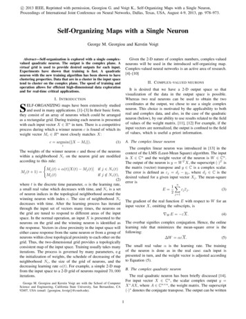
Journal of Statistical SoftwarePrediction of temperaturesPrediction of water content 0.6 0.50.4 0.3 0.2 0.1 70 6050 940 30 Figure 3: Supervised SOMs for the NIR data. The left plot shows the mapping of spectrawhen the XYF map has been trained with the water content as the y-variable; the radiusof the circles indicate the temperature at which spectra have been measured. The right plotdoes the opposite: temperature is used as y-variable and is visualized using the backgroundcolors, and the radii of the circles indicate water content.of the circles indicate the units onto which samples have been mapped – thus indicating anestimation of the water content – and the circle radii indicate measurement temperatures. Theright plot shows the reverse situation: there, the map has been trained to predict temperature.Thus, the position of a circle says something about the expected temperature at which thatsample has been measured, and the water concentration is indicated by the circle radius. Thisplot is obtained using the following code (adapted from the manual page of the xyf function):R water.predict - predict(nir.xyf) unit.predictionR temp.xyf - predict(nir.xyf2) unit.predictionR temp.predict - as.numeric(classmat2classvec(temp.xyf))R R R R R par(mfrow c(1, 2))plot(nir.xyf, type "property", property water.predict,main "Prediction of water content", keepMargins TRUE)scatter - matrix(rnorm(length(temperature)*2, sd .1), ncol 2)radii - (temperature - 20)/250symbols(nir.xyf grid pts[nir.xyf unit.classif,] scatter,circles radii, inches FALSE, add TRUE)R plot(nir.xyf2, type "property", property temp.predict, palette.name rainbow, main "Prediction of temperatures")R scatter - matrix(rnorm(nrow(composition)*2, sd .1), ncol 2)
10kohonen: Self- and Super-organizing Maps in RYX3040506070Figure 4: Plots of codebook vectors for the xyf mapping of IR spectra (X) and temperature(Y ).R radii - 0.05 0.4 * composition[,2]R symbols(nir.xyf2 grid pts[nir.xyf2 unit.classif,] scatter, circles radii, inches FALSE, add TRUE)The plot functions themselves use the property argument to show the unit predictions ina background color; we have chosen a different palette in the second plot to distinguish alsographically between the prediction of a continuous variable in the left plot and a categoricalvariable in the right plot. Circles are added using the symbols function. Their locationcontains two components: first, the position of the unit onto which a sample is mapped(contained in the unit.classif list element), and, second, a random component within thatunit. The keepMargins TRUE argument, which prevents the original graphical parametersfrom being restored is needed here (the plotting functions may change margins, for example,to accomodate all units in the figure and allow for a title or a legend), since the circles need tobe added to the correct position in the figure. Another application of setting keepMargins TRUE is to find out the unit number by the combination of the identify function and clickingthe map.The plots in Figure 3 show that the modelled parameter, indicated with the backgroundcolors, indeed has a spatially smooth (or coherent) distribution. Moreover, in the predictionof the water content (the left plot in the figure), the samples are ordered in such a waythat the low temperatures (the small circles) are located close together, as are the samplesmeasured at high temperatures. In the right plot, this is even more clear. Within one color(one measurement temperature), there is a gradient of water concentrations.In Figure 4 another use of the codebook vectors is shown. The R code to generate these
Journal of Statistical Software11figures is quite simple:R par(mfrow c(1, 2))R plot(nir.xyf2, "codes")For large numbers of variables, the default behaviour is to make a line plot rather than asegment plot, which leads to the spectra-like patterns to the left. By comparing the codebookvectors with Figure 3 we can immediately associate spectral features with water content. Inthe right plot, the codebook vectors of the dependent variable (in this case the categoricaltemperature variable) are shown. These can be directly interpreted as an indication of howlikely a given class is at a certain unit. Note that in some cases, such as at the boundariesbetween the higher temperatures, the classification of a unit is pretty uncertain.4.3. Super-organized maps: Data fusion with supersomInstead of one set of independent variables and one set of dependent variables, one may haveseveral data types for every object. The super-organized map introduced here accounts forindividual data types by using a separate layer for every type. Thus, when three types ofspectroscopy have been performed on a set of samples for which class information is presentas well, we could train a map using four layers. The first three would be continuous, and thecodebook vectors for these maps would resemble spectra, and the fourth would be discretewhere the codebook vectors can be interpreted as class memberships. A weight is associatedto every layer to be able to define an overall distance of an object to a unit. Again, thisallows much more flexibility than just concatenating the individual vectors corresponding tothe different data entitites for every sample. Obvious choices for the weights are to set themall equal (the default in the kohonen package), or to set them according to the number ofvariables in the indicidual data sets.We show an example, based on the well-known yeast cell-cycle data of Spellman et al. (1998).The mapping of these data, based on the four synchronisation methods with the largestnumbers of time points, is shown in Figure 5. The yeast data set, included in the kohonenpackage, are already in the correct form: a list where each element is a data matrix with onerow per gene. Note that the numbers of variables in the matrices need not be equal. The Rcode to generate the plot is as follows:R data(yeast)R set.seed(7)R yeast.supersom - supersom(yeast, somgrid(8, 8, "hexagonal"), whatmap 3:6)Warning message:removing 45 NA objects from the training datain: supersom(yeast, somgrid(8, 8, "hexagonal"), whatmap 3:6)R classes - levels(yeast class)R colors - c("yellow", "green", "blue", "red", "orange")R par(mfrow c(3, 2))R plot(yeast.supersom, type "mapping", pch 1, main "All", keepMargins TRUE)R for (i in seq(along classes)) {
12kohonen: Self- and Super-organizing Maps in RAll G2M S G1 M/G1 Figure 5: Mapping of the 80
of objects can be quite tedious. Moreover, there is no simple way to project new objects into the same space. Self-organizing maps (SOMs, Kohonen 2001) tackle the problem in a way similar to MDS, but instead of trying to reproduce distances they aim at reproducing topology,

![arXiv:1709.05254v2 [cs.LG] 1 Aug 2018 - University of St. Gallen](/img/34/gtc-2018-final.jpg)