Transcription
Euler Equation ErrorsMartin LettauSydney C. LudvigsonNew York University, CEPR, NBERNew York University and NBERPRELIMINARYComments WelcomeFirst draft: September 1, 2004This draft: February 5, 2005Lettau: Department of Finance, Stern School of Business, New York University, 44 West Fourth Street,New York, NY 10012-1126; Email: mlettau@stern.nyu.edu, Tel: (212) 998-0378; Fax: (212) 995-4233;http://www.stern.nyu.edu/ mlettau. Ludvigson: Department of Economics, New York University, 269Mercer Street, 7th Floor, New York, NY 10003; Email: sydney.ludvigson@nyu.edu, Tel: (212) 998-8927;Fax: (212) 995-4186; http://www.econ.nyu.edu/user/ludvigsons/. Ludvigson acknowledges nancialsupport from the Alfred P. Sloan Foundation and the CV Starr Center at NYU. We are grateful to DaveBackus, John Y. Campbell, George Constantinides, Mark Gertler, Stephen Gordon, Fatih Guvenen, StijnVan Nieuwerburgh, Martin Weitzman and seminar participants at New York University, Unversité Laval, andWest Virginia University for helpful comments. We Thank Jack Favalukis for excellent research assistance.Any errors or omissions are the responsibility of the authors.
Euler Equation ErrorsAbstractAmong the most important pieces of empirical evidence against the standard representativeagent, consumption-based asset pricing paradigm are the formidable unconditional Eulerequation errors the model produces for a broad stock market index return and short-terminterest rate. Unconditional Euler equation errors are also large for a broader cross-sectionof returns. Here we ask whether calibrated leading asset pricing models— speci cally developed to address empirical puzzles associated with the standard paradigm— explain theseempirical facts. We nd that, in many cases, they do not. We present several results. First,we show that if the true pricing kernel that sets the unconditional Euler equation errors tozero is jointly lognormally distributed with aggregate consumption and returns, then values for the subjective discount factor and relative risk aversion can always be found forwhich the standard model generates identical unconditional asset pricing implications fortwo asset returns, a risky and risk-free asset. Second, we show, using simulated data fromseveral leading asset pricing frameworks, that many economic models share this propertyeven though in those models the pricing kernel, returns, and consumption are not jointlylognormally distributed. Third, in contrast to the above results, we provide an exampleof a limited participation/incomplete markets model that is broadly consistent with theseempirical facts.JEL: G12, G10.
1IntroductionAmong the most important pieces of empirical evidence against the standard representativeagent, consumption-based asset pricing paradigm are the formidable unconditional Eulerequation errors the model produces for a broad stock market index return and short-term interest rate. Our de nition of the standard model assumes that agents have unrestricted accessto nancial markets, that assets can be priced using the Euler equations of a representativeconsumer maximizing the discounted value of power utility functions, and that the pricingkernel M , or stochastic discount factor, is equal to the marginal rate of substitution inconsumption. This model takes the formE [Mt Rt ] 1;Mt (Ct Ct 1 );(1)where Rt denotes the gross return on any tradable asset, Ct is per capita aggregate consumption,is the coe cient of relative risk-aversion andis a subjective time-discount factor.The average Euler equation errors are also large for a broader cross-section of returns thatincludes size and book-market sorted portfolio returns.We argue that these Euler equation errors constitute a puzzle for the standard consumptionbased asset pricing model that is at least as damning as other, more well known, conundrumsthat have received far more attention, such as the equity premium puzzle, risk-free rate puzzle, and time-series predictability of excess stock market returns. We employ these empiricalfacts to evaluate leading asset pricing models that have been speci cally developed to address puzzles generated by the standard paradigm (1). If leading asset pricing models aretrue, then in these models using (1) to price assets should generate large unconditional assetpricing errors, as in the data. The underlying assumption in each of these leading modelsis that, by discarding the standard pricing kernel in favor of the true kernel implied by themodel, an econometrician would be better able to model asset pricing data.In this paper we show that this is not always the case. Often, in leading asset pricingmodels, a standard representative-agent “pricing kernel” based on (1) can be found thathas virtually identical unconditional pricing implications for speci c asset returns, such as arisky asset and risk-free asset, or for a larger cross-section of risky asset returns. Thus, aneconometrician who observed data generated from any number of these leading models wouldfail to reject the standard consumption-based model in tests of its unconditional momentrestrictions, let alone replicate the sizable unconditional Euler equation errors found when tting historical data to (1).The literature has already demonstrated that it is possible, in principle, to explain anyobserved behavior of per capita aggregate consumption and asset returns, by appealing to incomplete consumption insurance. Constantinides and Du e (1996) prove a set of theoretical1
propositions showing that any observed joint process of aggregate consumption and returnscan be an equilibrium outcome if the second moments of the cross-sectional distribution ofconsumption growth and asset returns covary in the right way. Krebs (2004) shows thatany observed joint process of aggregate consumption and asset returns can be rationalizedif all assetholders are subject to su ciently extreme idiosyncratic events with very smallprobability of occurrence. In this paper we move away from theoretical propositions and askwhether particular calibrated economies of leading asset pricing models are quantitativelycapable of matching the large unconditional Euler equation errors generated by the standardconsumption-based model when tted to data. This is important because it remains unclearwhether plausibly calibrated models built on primitives of tastes, technology, and underlyingshocks can in practice generate the joint behavior we observe in the data.Our analysis uses simulated data from several leading economic models designed addressempirical failures of the standard model (1). These models include the representative-agentexternal habit-persistence paradigms of (i) Campbell and Cochrane (1999) and (ii) Menzly,Santos, and Veronesi (2004), (iii) the representative-agent long-run risks model based onrecursive preferences of Bansal and Yaron (2004), and (iv) the limited participation modelof Guvenen (2003). Each is an explicitly parameterized economic model calibrated to accordwith the data in plausible ways, and each has proven remarkably successful in explaining arange of asset pricing phenomena. In addition to these models, we dig more deeply into theaggregate Euler equation implications of simple asset pricing models with limited participation/incomplete markets, in which assetholder consumption is permitted to behave quitedi erently from per capita aggregate consumption.Our focus on Euler equations is intentional, since they represent the set of theoreticalrestrictions from which all asset pricing implications follow. Formal econometric tests ofconditional Euler equations using aggregate consumption data lead to rejections of the standard representative-agent, consumption-based asset pricing model, even when no bounds areplaced on the coe cient of relative risk aversion or the rate of time preference (Hansen andSingleton (1982); Ferson and Constantinides (1991); Hansen and Jagannathan (1991)). Similarly, we show here that the quarterly pricing errors for the unconditional Euler equationsassociated with an aggregate equity return and a short-term Treasury bill rate are large when tting aggregate data to (1), even when the coe cient of relative risk aversion or the rate oftime preference are left unrestricted and chosen to minimize those errors. For larger crosssections of returns the results are similar. These empirical results place additional testablerestrictions on asset pricing models: not only must such models have zero pricing errorswhen the pricing kernel is correctly speci ed according to the model, they must also producelarge pricing errors when the pricing kernel is incorrectly speci ed using power utility andaggregate consumption, even whenandare chosen to minimize those errors.2
Our main ndings are as follows:First, we show that if the true pricing kernel that sets Euler equation errors to zero isjointly lognormally distributed with aggregate consumption and returns, then values for thediscount factor and relative risk aversion can be always be found for which the standard modelgenerates identical unconditional asset pricing implications for two asset returns, a risky andrisk-free asset. This property implies that such models will not be capable of explaining theempirical facts discussed above, namely the large Euler equation errors found when assetreturn data are tted to (1). We illustrate these results in an incomplete markets/limitedparticipation setting.Second, using simulated data from each of the leading asset pricing models mentionedabove, we show that many economic models share this property even though in these modelsthe pricing kernel, returns, and consumption are not jointly lognormally distributed. Some ofthe models we study can explain why an econometrician obtains implausibly high estimatesofandwhen freely tting aggregate data to (1). But, they cannot explain the largeunconditional Euler equation errors associated with such estimates. The asset pricing modelswe consider counterfactually imply that values for the subjective discount factor and riskaversion can be found for which (1) satis es the unconditional Euler equation restrictionsjust as well as the true pricing kernel.Third, in contrast to the above results, we provide one example in an incomplete markets/limited participation setting of a model that can roughly replicate the empirical facts,if the joint distribution of aggregate consumption, individual assetholder consumption, andstock returns takes a particular form of deviations from normality. But we also nd—within this broad class of distributions we consider— that many non-normal distributionspeci cations do not explain the sizeable Euler equation errors generated by the standardconsumption-based asset pricing model (1). Similar ndings hold for the average Eulerequation errors over a larger cross-section of asset returns.We emphasize that this paper is not a criticism of work that investigates the asset pricingimplications of models with preferences or market structures that di er from the standardconsumption-based model. Indeed, we view our paper as a compliment to the existingliterature because it provides a di erent perspective on whether such models are capable offully rationalizing the joint behavior of asset prices and aggregate quantities. We also addto the literature by outlining the econometric consequences, for estimation and testing ofunconditional Euler equations, of tting the standard pricing kernel (1) to data when thetrue pricing kernel that generated the data is derived from some other model. Finally, westress that our results do not imply that no model can be made consistent with the testablerestrictions we focus on here— we present an incomplete markets example to the contrary.Our point is that many models, including those at the forefront of asset pricing theory, do3
not satisfy these testable restrictions.The rest of this paper is organized as follows. The next section lays out the empiricalEuler equation facts using post-war U.S. data on per capita aggregate consumption andreturns. Section 3 studies the implications of various economic theories for the same Eulerequation errors we measure in the data. We begin with a simple example in which the truepricing kernel is jointly lognormally distributed with aggregate consumption growth and assetreturns. Next, we investigate the extent to which leading asset pricing models, calibratedto accord with the U.S. data, are capable of explaining the empirical facts. Here we focusboth on the case of a single risky and a risk-free asset return and on models that exploita larger cross-section of risky returns. Our main ndings are shown to be robust to timeaggregation of aggregate consumption data, and to the introduction of limited participationin the representative-agent models. Finally, we provide one example of a simple incompletemarkets/limited participation model that can roughly replicate the empirical Euler equationerrors from historical data. Section 4 concludes.2Euler Equation Errors: The FactsIn this section we document empirical facts of the standard consumption-based asset pricingmodel that pertain to unconditional Euler equations using aggregate consumption.The standard consumption based model, as de ned above, has the following characteristics. There exists representative-consumer with constant relative risk aversion (CRRA)preferences over consumption given by(1XU Et 01t Ct11where Ct is per capita aggregate consumption,);(2) 0;is a subjective time-discount factor, andis the coe cient of relative risk aversion. At each date, agents maximize (2) subject toan accumulation equation for wealth that links assets today to returns today and savingsyesterday. Agents have unrestricted access to nancial markets; they face no borrowingor short-sales constraints. The asset pricing model comes from the rst-order conditionsfor optimal consumption choice, which place restrictions on the joint distribution of theintertemporal marginal rate of substitution in consumption, given by Mt 1(Ct 1 Ct );and asset returns. The rst-order conditions imply that for any traded asset indexed by j,jwith a gross return at time t 1 of Rt 1; the following set of Euler equation holds:jEt Mt 1 Rt 1 1:4(3)
Here Et is the conditional expectation operator, conditional on time t information. Themarginal rate of substitution in consumption, Mt 1 , is the stochastic discount factor, orpricing kernel.By the law of iterated expectations, equation (3) also implies the following set of unconditional Euler equations that must hold for any traded asset indexed by j :jE Mt 1 Rt 1 1;(4)where E is the unconditional expectation operator.We refer to the di erence between the left-hand-side of (4) and unity as the unconditionalEuler equation error, or alternatively the pricing error, associated with the jth asset return:Pricing error of asset j E(Ct Ct 1 )jRt 11:If the standard model is true then these errors should be zero for any traded asset, givensome values of the parametersand .We focus much of our attention on the unconditional Euler equation errors associatedwith two asset returns: a broad stock market index return (measured as the the CRSPvalue-weighted price index return and denoted Rts ) and short-term “riskless” interest rate(measured as the three-month Treasury bill rate and denoted Rtf ). We maintain this focusfor two reasons. First, the standard model’s inability to explain properties of just thesetwo returns has been central to the development of a consensus that the model is seriously‡awed. Second, all asset pricing models seek to match the empirical properties of these tworeturns and most generate no implications for larger cross-sections of securities because thecash ‡ow properties of these securities are not modeled. Nevertheless, we also consider theEuler equation errors associated with a broader cross-section of returns, including portfolioreturns formed on the basis of size and book-market ratios. Notice that estimation of (4) forthe two-asset case collapses to an excercise in solving two nonlinear equations. In this case,the vector of sample pricing errors contains no nondegenerate random variables and thus thepricing errors are not a ected by sampling error.There are several ways to present the pricing errors implied by the standard consumptionbased model for these two asset returns. One is to combine the separate Euler equations forthe stock market return and Treasury bill rate into a single Euler equation for the excessreturn that is a function of only the risk aversion parameter . From (4) we have"#Ct 1fsERt 1Rt 1 0:Ct(5)The empirical pricing error for the excess return is given by an estimate of the left-hand-sideof (5). Figure 1 plots this error over a range of values of , where the error is computed as5
the sample mean of the expression in square brackets in (5). The estimation uses quarterly,per capita data on nondurables and services expenditures measured in 1996 dollars as ameasure of consumption Ct , in addition to the return data mentioned above.1 Returns arede‡ated by the implicit price de‡ator corresponding to the measure of consumption Ct . Thedata span the period from the rst quarter of 1951 to the fourth quarter of 2002. A detaileddescription is provided in the Appendix.Figure 1 shows that the pricing error (5) cannot be driven to zero, or indeed even to asmall number, for any value of . The lowest pricing error is almost 4% per annum, whichoccurs at 117. This pricing error is almost half of the average annual CRSP stock returnand four times the average annual Treasury-bill rate. At other values ofthis error risesprecipitously and reaches several times the average annual stock market return whenoutside the ranges displayed in Figure 1. Thus, there is no value ofisthat sets the pricing2error (5) to zero.Another way to present the pricing errors implied by the standard model for the stockmarket return and Treasury bill rate is to choose values forandthat make the estimatedEuler equation errors for each asset return as close as possible to the theoretical Eulerequation errors of zero:EE""Ct 1CtsRt 1Ct 1CtfRt 1##1 01 0:This amounts to solving two (nonlinear) equations in two unknowns,choose parameters for time preferenceand risk aversionand . To do so, weto minimize a weighted sum ofsquared pricing errors, an application of exactly identi ed Generalized Method of Moments(GMM, Hansen (1982)):min gT ( ; ) ! s E;(Ct Ct 1 )for some weights ! s and ! f . LetcandRtsc12 !f Eh(Ct Ct 1 )Rtfi21 ;denote the arg min gT ( ; ), the values ofandthat minimize the scalar gT ( ; ).Panel A of Table 1 shows that when the risk aversion and time preference parametersare chosen to minimize an equally weighted sum of squared pricing errors (! s ! f 1),the pricing errors for the stock market return and the short-term Treasury bill rate are splitevenly, with each error close to 2.7% per annum for the stock market return and close to12We exclude shoes and clothing expenditure from this series since they are partly durable.Note that (5) is a nonlinear function of : Thus, there is not necessarily a solution.6
-2.7% for the Treasury bill. As before, this magnitude is large: it is about one-third of theaverage annual stock market return, and about three times as large as the average annualTreasury bill return. The last column shows that the square root of the average squaredpricing error is 60% of the cross-sectional mean return for these two assets. Naturally, whenwe place 100 times more weight on the Euler equation associated with the stock market returnin this minimization (! s 100; ! f 1), the pricing error associated with the stock returncan be made close to zero, but then the error associated with the Treasury bill explodes to-5.4% per annum. Conversely, when we place 100 times more weight on the Euler equationassociated with the Treasury bill rate (! s 1; ! f 100), the pricing error associated withthe Treasury bill can be made close to zero, but the error associated with the stock returnrises to 5.4% per annum. Thus, there are no values ofzero. Regardless of the particular weighting scheme,andcandthat set the pricing errors toc(which are left unrestricted)are close to 1.4 and 90, respectively.Figure 2 displays the (negative of) the square root of the averaged squared pricing errorsover a range of values forand . The gure is presented this way for ease of readability.The pricing errors are obviously smallest at the point estimates forand , but the gureshows that they are large over a wide range of values for these parameters. Finally, Figure3 shows the contour plots for the output displayed in Figure 2. The gures show that thereis no combination of parameter values forandfor which the pricing errors of both assetreturns can be set to zero, or even small in magnitude.Why are the pricing errors for the stock return and Treasury-bill rate so large? Panel Bof Table 1 provides a partial answer: a large part (but not all) of the unconditional Eulerequation errors generated by this model are associated with recessions, periods in whichper capita aggregate consumption growth is steeply negative. If we remove the data pointsassociated with the smallest six observations on consumption growth, the equally weightedpricing errors are 0.7% for the stock market return and -0.7% for the Treasury-bill rate,a 74% reduction. Table 2 identi es these six observations as they are located throughoutthe sample. Each occur in the depths of recessions in the 1950s, 1970s, early 1960s, 1980sand 1990s, as identi ed by the National Bureau of Economic Research. In these periods,aggregate per capita consumption growth is steeply negative but the aggregate stock returnand Treasury-bill rate is, more often than not, steeply positive. Since the product of themarginal rate of substitution and the gross asset return must be unity on average, suchnegative comovement (positive comovement between Mt and returns) contributes to largepricing error. One can also reduce the (equally-weighted) pricing errors by using annualreturns and year-over-year consumption growth (fourth quarter over fourth quarter).3 This3Jagannathan and Wang (2004) study the ability of the standard model to explain a large cross-section7
procedure averages out the worst quarters for consumption growth instead of removing them.Either procedure eliminates much of the cyclical variation in consumption. To see this, notethat on a quarterly basis the largest declines in consumption are about six times as large atan annual rate as those on a year-over-year basis.Of course, these quarterly episodes are not outliers to be ignored, but signi cant economicevents to be explained. Indeed, we argue that such Euler equation errors–driven by periodsof important economic change–are among the most damning pieces of evidence against thestandard model. An important question is why the standard model performs so poorly inrecessions relative to other times.The pricing error of the Euler equation associated with the stock market return is alwayspositive implying a positive “alpha” in the expected return-beta representation. This saysthat unconditional risk premia are too high to be explained by the stock market’s covariancewith the marginal rate of substitution of aggregate consumption, a familiar result from theequity premium literature.4 The high alphas generated by the standard consumption-basedmodel constitute one of the most remarked-upon failures in the history of asset pricingtheory.What about larger cross-sections of returns? Panel B of Table 1 reports the pricingerrors for a cross-section of eight asset returns. The asset returns include as before theTreasury bill rate and CRSP stock market return, in addition to six value-weighted portfolioreturns of common stock sorted into two size (market equity) quantiles and three bookvalue-market value quantiles. These returns were taken from Professor Kenneth French’sDartmouth web page. The latter six portfolios are created from stocks traded on the NYSE,AMEX, and NASDAQ, as detailed on Kenneth French’s web page. We use equity returns onof asset returns using forth quarter over fourth quarter consumption growth and annual asset returns. They nd more support for the model when year-over-year growth rates are restricted to the fourth quarter.4The expected return-beta representation is derived from the Euler equationE [Mt Rts ]1 e;where e denotes the pricing error associated with the Euler equation. This equation can be rearranged toyieldCov (Mt ; Rts ) Var (Mt )eE (Rts ) 1 E (Mt ) ;Var (Mt )E (Mt )E (Mt )where 1 E (Mt ) is interpreted as the risk-free rate in models for which this rate is presumed constant.Rewrite the above asE (Rts ) 1 E (Mt ) ;where the left-hand-side is the risk-premium on the stock return,Var(Mt )E(Mt )Cov(Mt ;Rts )Var(Mt )is the “beta” for theis the price of risk associated with Mt , andstochastic discount factor Mt , or quantity of rn,that is the part of the risk-premium thatE(Mt )cannot be explained by its beta risk.8
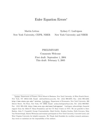
size and book-to-market sorted portfolios because Fama and French (1992) show that thesetwo characteristics provide a “simple and powerful characterization” of the cross-section ofaverage stock returns, and absorb the roles of leverage, earnings-to-price ratio and manyother factors governing cross-sectional variation in average stock returns. For this set ofasset returns parametersandare chosen to minimize the quadratic form gT ( ; )wT0( ; ) WwT ( ; ), where wT ( ; ) is the (8 1) vector of average pricing errors for eachPCtasset (i.e., wjT ( ; ) T1 Tt 1Rtj 1 for j 1; :::; 8) and W is the 8 8 identityCt 1matrix. We use the identity weighting matrix because we are interested in the average pricingerrors for these particular returns, which Fama and French show are based on economicallyinteresting characteristics and deliver a wide spread in cross-sectional average returns. Usingthe optimal GMM weighting matrix (for example) would require us to minimize the pricingerrors for re-weighted portfolios of the original test assets.Panel B shows that the square root of the average squared pricing error (RMSE) for theeight asset returns is large: over three% on an annual basis, or over 35% of the cross-sectionalaverage mean return. Eliminating the lowest six consumption growth rate periods reducesthe average pricing errors, but they remain large, around 2% on an annual basis.How much might sampling error alone contribute to the estimated Euler equation errorsfor the stock return and Treasury bill rate? In principle, this question can be addressed inexactly identi ed systems by conducting a block bootstrap simulation of the raw data. Thisapproach is inappropriate for the application here, however, because such a procedure woulde ectively treat the low consumption growth periods in our sample as outliers, in the sensethat a nontrivial fraction of the simulated samples would exclude those observations. But aswe have argued above, these episodes of low or negative consumption growth— the hallmarkof recessions— are not outliers to be ignored, but signi cant economic events to be explained.A more appropriate approach to this question is to ask, given sampling error, how likelyis it that we would observe the pricing errors we observe under the null hypothesis thatthe standard model is true and the Euler equations are exactly satis ed in population?Models that postulate joint lognormality for consumption and asset returns are null modelsof this form, since in this case values forandalways exist for which the populationEuler equations of any two asset returns are exactly satis ed. Consequently, only samplingerror in the estimated Euler equations could cause non-zero pricing errors. It is thereforenatural to begin by assessing whether joint lognormality is a plausible description of ourconsumption and return data, once we take into account sampling error. We do so byperforming formal statistical tests of lognormality in our data. Table 3 presents the resultsof normality tests, based on estimates of both univariate and multivariate skewness andkurtosis for log (Ct Ct 1 )ct ; log (Rst )rst , and log (Rf t )9rf t .
There is strong evidence against normality from both univariate and multivariate tests.We reject that skewness is zero at the one% or better level forof the three variablesct , and rst , for every pairct , rst , and rf t ; and for the triple ( ct ; rst ; rf t ) : Also at better thanthe one% level, we may reject the null hypothesis that the kurtosis measures for any threeofct , rst , and rf t are equal to those of a univariate normal distribution, and that thekurtosis measure for any pair of these variable or for the triple ( ct ; rst ; rf t ) is equal to thatof a multivariate normal distribution. The same picture emerges from examining quantilequantile plots (QQ plots) forct , rst , and rf t and for the three variables jointly, givenin Figure 4. This gure plots the sample quantiles for the data against those that wouldarise under the null of joint lognormality. Pointwise standard error bands are computed bysimulating from the appropriate distribution with length equal to the size of our data set.The gure shows that all three log variables have some quantiles that lie outside the standarderror bands for univariate normality. But the most dramatic departure from normality isdisplayed in the multivariate QQ plot for the joint distribution of ( ct ; rst ; rf t ). In this case,a vast range of quantiles lie far outside the standard error bands for joint normality.We address the issue of sampling error in our application from another angle. Supposethat the data were generated by the standard CRRA representative-agent model, with returns and consumption jointly lognormally distributed. How likely is it that we would
equation errors the model produces for a broad stock market index return and short-term interest rate. Unconditional Euler equation errors are also large for a broader cross-section of returns. Here we ask whether