Transcription
31216.416. Particle Swarm OptimizationBasic PSO ParametersThe basic PSO is influenced by a number of control parameters, namely the dimensionof the problem, number of particles, acceleration coefficients, inertia weight, neighborhood size, number of iterations, and the random values that scale the contributionof the cognitive and social components. Additionally, if velocity clamping or constriction is used, the maximum velocity and constriction coefficient also influence theperformance of the PSO. This section discusses these parameters.The influence of the inertia weight, velocity clamping threshold and constriction coefficient has been discussed in Section 16.3. The rest of the parameters are discussedbelow: Swarm size, ns , i.e. the number of particles in the swarm: the more particlesin the swarm, the larger the initial diversity of the swarm – provided that agood uniform initialization scheme is used to initialize the particles. A largeswarm allows larger parts of the search space to be covered per iteration. However, more particles increase the per iteration computational complexity, andthe search degrades to a parallel random search. It is also the case that moreparticles may lead to fewer iterations to reach a good solution, compared tosmaller swarms. It has been shown in a number of empirical studies that thePSO has the ability to find optimal solutions with small swarm sizes of 10 to 30particles [89, 865]. Success has even been obtained for fewer than 10 particles[863]. While empirical studies give a general heuristic of ns [10, 30], the optimal swarm size is problem-dependent. A smooth search space will need fewerparticles than a rough surface to locate optimal solutions. Rather than usingthe heuristics found in publications, it is best that the value of ns be optimizedfor each problem using cross-validation methods. Neighborhood size: The neighborhood size defines the extent of social interaction within the swarm. The smaller the neighborhoods, the less interactionoccurs. While smaller neighborhoods are slower in convergence, they have morereliable convergence to optimal solutions. Smaller neighborhood sizes are lesssusceptible to local minima. To capitalize on the advantages of small and largeneighborhood sizes, start the search with small neighborhoods and increase theneighborhood size proportionally to the increase in number of iterations [820].This approach ensures an initial high diversity with faster convergence as theparticles move towards a promising search area. Number of iterations: The number of iterations to reach a good solution is alsoproblem-dependent. Too few iterations may terminate the search prematurely.A too large number of iterations has the consequence of unnecessary addedcomputational complexity (provided that the number of iterations is the onlystopping condition). Acceleration coefficients: The acceleration coefficients, c1 and c2 , togetherwith the random vectors r1 and r2 , control the stochastic influence of the cognitive and social components on the overall velocity of a particle. The constantsc1 and c2 are also referred to as trust parameters, where c1 expresses how much
16.4 Basic PSO Parameters313confidence a particle has in itself, while c2 expresses how much confidence a particle has in its neighbors. With c1 c2 0, particles keep flying at their currentspeed until they hit a boundary of the search space (assuming no inertia). Ifc1 0 and c2 0, all particles are independent hill-climbers. Each particle findsthe best position in its neighborhood by replacing the current best position ifthe new position is better. Particles perform a local search. On the other hand,if c2 0 and c1 0, the entire swarm is attracted to a single point, ŷ. Theswarm turns into one stochastic hill-climber.Particles draw their strength from their cooperative nature, and are most effective when nostalgia (c1 ) and envy (c2 ) coexist in a good balance, i.e. c1 c2 . Ifc1 c2 , particles are attracted towards the average of yi and ŷ [863, 870]. Whilemost applications use c1 c2 , the ratio between these constants is problemdependent. If c1 c2 , each particle is much more attracted to its own personalbest position, resulting in excessive wandering. On the other hand, if c2 c1 ,particles are more strongly attracted to the global best position, causing particles to rush prematurely towards optima. For unimodal problems with a smoothsearch space, a larger social component will be efficient, while rough multi-modalsearch spaces may find a larger cognitive component more advantageous.Low values for c1 and c2 result in smooth particle trajectories, allowing particlesto roam far from good regions to explore before being pulled back towards goodregions. High values cause more acceleration, with abrupt movement towards orpast good regions.Usually, c1 and c2 are static, with their optimized values being found empirically.Wrong initialization of c1 and c2 may result in divergent or cyclic behavior[863, 870].Clerc [134] proposed a scheme for adaptive acceleration coefficients, assumingthe social velocity model (refer to Section 16.3.5):c2 (t) c2,max c2,mine mi (t) 1c2,min c2,max m (t)22e i 1(16.35)where mi is as defined in equation (16.30). The formulation of equation (16.30)implies that each particle has its own adaptive acceleration as a function of theslope of the search space at the current position of the particle.Ratnaweera et al. [706] builds further on a suggestion by Suganthan [820] to linearly adapt the values of c1 and c2 . Suganthan suggested that both accelerationcoefficients be linearly decreased, but reported no improvement in performanceusing this scheme [820]. Ratnaweera et al. proposed that c1 decreases linearlyover time, while c2 increases linearly [706]. This strategy focuses on explorationin the early stages of optimization, while encouraging convergence to a goodoptimum near the end of the optimization process by attracting particles moretowards the neighborhood best (or global best) positions. The values of c1 (t)and c2 (t) at time step t is calculated ast c1,maxnttc2 (t) (c2,max c2,min ) c2,minntc1 (t) (c1,min c1,max )(16.36)(16.37)
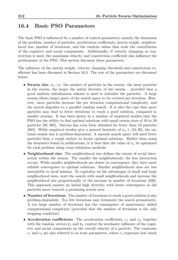
31416. Particle Swarm Optimizationwhere c1,max c2,max 2.5 and c1,min c2,min 0.5.A number of theoretical studies have shown that the convergence behavior of PSO issensitive to the values of the inertia weight and the acceleration coefficients [136, 851,863, 870]. These studies also provide guidelines to choose values for PSO parametersthat will ensure convergence to an equilibrium point. The first set of guidelines areobtained from the different constriction models suggested by Clerc and Kennedy [136].For a specific constriction model and selected φ value, the value of the constrictioncoefficient is calculated to ensure convergence.For an unconstricted simplified PSO system that includes inertia, the trajectory of aparticle converges if the following conditions hold [851, 863, 870, 937]:1 w 1(φ1 φ2 ) 1 02(16.38)and 0 w 1. Since φ1 c1 U (0, 1) and φ2 c2 U (0, 1), the acceleration coefficients,c1 and c2 serve as upper bounds of φ1 and φ2 . Equation (16.38) can then be rewrittenas1(16.39)1 w (c1 c2 ) 1 02Therefore, if w, c1 and c2 are selected such that the condition in equation (16.39)holds, the system has guaranteed convergence to an equilibrium state.The heuristics above have been derived for the simplified PSO system with no stochastic component. It can happen that, for stochastic φ1 and φ2 and a w that violatesthe condition stated in equation (16.38), the swarm may still converge. The stochastictrajectory illustrated in Figure 16.6 is an example of such behavior. The particle follows a convergent trajectory for most of the time steps, with an occasional divergentstep.Van den Bergh and Engelbrecht show in [863, 870] that convergent behavior will beobserved under stochastic φ1 and φ2 if the ratio,φratio φcritc1 c2(16.40)is close to 1.0, whereφcrit sup φ 0.5 φ 1 w,φ (0, c1 c2 ](16.41)It is even possible that parameter choices for which φratio 0.5, may lead to convergentbehavior, since particles spend 50% of their time taking a step along a convergenttrajectory.16.5Single-Solution Particle Swarm OptimizationInitial empirical studies of the basic PSO and basic variations as discussed in this chapter have shown that the PSO is an efficient optimization approach – for the benchmark
16.5 Single-Solution Particle Swarm 50tFigure 16.6 Stochastic Particle Trajectory for w 0.9 and c1 c2 2.0problems considered in these studies. Some studies have shown that the basic PSOimproves on the performance of other stochastic population-based optimization algorithms such as genetic algorithms [88, 89, 106, 369, 408, 863]. While the basic PSOhas shown some success, formal analysis [136, 851, 863, 870] has shown that the performance of the PSO is sensitive to the values of control parameters. It was also shownthat the basic PSO has a serious defect that may cause stagnation [868].A variety of PSO variations have been developed, mainly to improve the accuracy ofsolutions, diversity and convergence behavior. This section reviews some of these variations for locating a single solution to unconstrained, single-objective, static optimization problems. Section 16.5.2 considers approaches that differ in the social interactionof particles. Some hybrids with concepts from EC are discussed in Section 16.5.3.Algorithms with multiple swarms are discussed in Section 16.5.4. Multi-start methodsare given in Section 16.5.5, while methods that use some form of repelling mechanismare discussed in Section 16.5.6. Section 16.5.7 shows how PSO can be changed to solvebinary-valued problems.Before these PSO variations are discussed, Section 16.5.1 outlines a problem with thebasic PSO.
31616.5.116. Particle Swarm OptimizationGuaranteed Convergence PSOThe basic PSO has a potentially dangerous property: when xi yi ŷ, the velocityupdate depends only on the value of wvi . If this condition is true for all particlesand it persists for a number of iterations, then wvi 0, which leads to stagnation ofthe search process. This point of stagnation may not necessarily coincide with a localminimum. All that can be said is that the particles converged to the best positionfound by the swarm. The PSO can, however, be pulled from this point of stagnationby forcing the global best position to change when xi yi ŷ.The guaranteed convergence PSO (GCPSO) forces the global best particle to searchin a confined region for a better position, thereby solving the stagnation problem[863, 868]. Let τ be the index of the global best particle, so thatyτ ŷ(16.42)GCPSO changes the position update toxτ j (t 1) ŷj (t) wvτ j (t) ρ(t)(1 2r2 (t))(16.43)which is obtained using equation (16.1) if the velocity update of the global best particlechanges tovτ j (t 1) xτ j (t) ŷj (t) wvτ j (t) ρ(t)(1 2r2j (t))(16.44)where ρ(t) is a scaling factor defined in equation (16.45) below. Note that only theglobal best particle is adjusted according to equations (16.43) and (16.44); all otherparticles use the equations as given in equations (16.1) and (16.2).The term xτ j (t) in equation (16.44) resets the global best particle’s position to theposition ŷj (t). The current search direction, wvτ j (t), is added to the velocity, andthe term ρ(t)(1 2r2j (t)) generates a random sample from a sample space with sidelengths 2ρ(t). The scaling term forces the PSO to perform a random search in an areasurrounding the global best position, ŷ(t). The parameter, ρ(t) controls the diameterof this search area, and is adapted using if #successes(t) s 2ρ(t)0.5ρ(t) if #f ailures(t) f(16.45)ρ(t 1) ρ(t)otherwisewhere #successes and #f ailures respectively denote the number of consecutive successes and failures. A failure is defined as f (ŷ(t)) f (ŷ(t 1)); ρ(0) 1.0 was foundempirically to provide good results [863, 868]. The threshold parameters, s and fadhere to the following conditions:#successes(t 1)#f ailures(t 1) #successes(t) #f ailures(t 1) 0#f ailures(t) #successes(t 1) 0(16.46)(16.47)The optimal choice of values for s and f is problem-dependent. Van den Bergh et al.[863, 868] recommends that s 15 and f 5 be used for high-dimensional search
16.5 Single-Solution Particle Swarm Optimization317spaces. The algorithm is then quicker to punish poor ρ settings than it is to rewardsuccessful ρ values.Instead of using static s and f values, these values can be learnt dynamically. Forexample, increase sc each time that #f ailures f , which makes it more difficultto reach the success state if failures occur frequently. Such a conservative mechanismwill prevent the value of ρ from oscillating rapidly. A similar strategy can be used for s .The value of ρ determines the size of the local area around ŷ where a better positionfor ŷ is searched. GCPSO uses an adaptive ρ to find the best size of the samplingvolume, given the current state of the algorithm. When the global best position isrepeatedly improved for a specific value of ρ, the sampling volume is increased toallow step sizes in the global best position to increase. On the other hand, when fconsecutive failures are produced, the sampling volume is too large and is consequentlyreduced. Stagnation is prevented by ensuring that ρ(t) 0 for all time steps.16.5.2Social-Based Particle Swarm OptimizationSocial-based PSO implementations introduce a new social topology, or change the wayin which personal best and neighborhood best positions are calculated.Spatial Social NetworksNeighborhoods are usually formed on the basis of particle indices. That is, assuminga ring social network, the immediate neighbors of a particle with index i are particleswith indices (i 1 mod ns ) and (i 1 mod ns ), where ns is the total number ofparticles in the swarm. Suganthan proposed that neighborhoods be formed on thebasis of the Euclidean distance between particles [820]. For neighborhoods of sizenN , the neighborhood of particle i is defined to consist of the nN particles closest toparticle i. Algorithm 16.4 summarizes the spatial neighborhood selection process.Calculation of spatial neighborhoods require that the Euclidean distance between allparticles be calculated at each iteration, which significantly increases the computational complexity of the search algorithm. If nt iterations of the algorithm is executed,the spatial neighborhood calculation adds a O(nt n2s ) computational cost. Determining neighborhoods based on distances has the advantage that neighborhoods changedynamically with each iteration.Fitness-Based Spatial NeighborhoodsBraendler and Hendtlass [81] proposed a variation on the spatial neighborhoods implemented by Suganthan, where particles move towards neighboring particles thathave found a good solution. Assuming a minimization problem, the neighborhood of
31816. Particle Swarm OptimizationAlgorithm 16.4 Calculation of Spatial Neighborhoods; Ni is the neighborhood ofparticle iCalculate the Euclidean distance E(xi1 , xi2 ), i1 , i2 1, . . . , ns ;S {i : i 1, . . . , ns };for i 1, . . . , ns do S S; for i 1, . . . , nNi do Ni Ni {xi : E(xi , xi ) min{E(xi , xi ), xi S }; S S \ {xi };endendparticle i is defined as the nN particles with the smallest value ofE(xi , xi ) f (xi )(16.48) where E(xi , xi ) is the Euclidean distance between particles i and i , and f (xi ) is the fitness of particle i . Note that this neighborhood calculation mechanism also allowsfor overlapping neighborhoods.Based on this scheme of determining neighborhoods, the standard lbest PSO velocity equation (refer to equation (16.6)) is used, but with ŷi the neighborhood-bestdetermined using equation (16.48).Growing NeighborhoodsAs discussed in Section 16.2, social networks with a low interconnection convergeslower, which allows larger parts of the search space to be explored. Convergence ofthe fully interconnected star topology is faster, but at the cost of neglecting partsof the search space. To combine the advantages of better exploration by neighborhood structures and the faster convergence of highly connected networks, Suganthancombined the two approaches [820]. The search is initialized with an lbest PSO withnN 2 (i.e. with the smallest neighborhoods). The neighborhood sizes are thenincreased with increase in iteration until each neighborhood contains the entire swarm(i.e. nN ns ).Growing neighborhoods are obtained by adding particle position xi2 (t) to the neighborhood of particle position xi1 (t) if xi1 (t) xi2 (t) 2 dmax(16.49)where dmax is the largest distance between any two particles, and 3t 0.6ntnt(16.50)
16.5 Single-Solution Particle Swarm Optimization319with nt the maximum number of iterations.This allows the search to explore more in the first iterations of the search, with fasterconvergence in the later stages of the search.Hypercube StructureFor binary-valued problems, Abdelbar and Abdelshahid [5] used a hypercube neighborhood structure. Particles are defined as neighbors if the Hamming distance betweenthe bit representation of their indices is one. To make use of the hypercube topology,the total number of particles must be a power of two, where particles have indicesfrom 0 to 2nN 1. Based on this, the hypercube has the properties [5]: Each neighborhood has exactly nN particles. The maximum distance between any two particles is exactly nN . If particles i1 and i2 are neighbors, then i1 and i2 will have no other neighborsin common.Abdelbar and Abdelshahid found that the hypercube network structure provides betterresults than the gbest PSO for the binary problems studied.Fully Informed PSOBased on the standard velocity updates as given in equations (16.2) and (16.6), eachparticle’s new position is influenced by the particle itself (via its personal best position) and the best position in its neighborhood. Kennedy and Mendes observed thathuman individuals are not influenced by a single individual, but rather by a statisticalsummary of the state of their neighborhood [453]. Based on this principle, the velocity equation is changed such that each particle is influenced by the successes of all itsneighbors, and not on the performance of only one individual. The resulting PSO isreferred to as the fully informed PSO (FIPS).Two models are suggested [453, 576]: Each particle in the neighborhood, Ni , of particle i is regarded equally. Thecognitive and social components are replaced with the termnNi r(t)(ym (t) xi (t))nNim 1(16.51)where nNi Ni , Ni is the set of particles in the neighborhood of particle ias defined in equation (16.8), and r(t) U (0, c1 c2 )nx . The velocity is thencalculated asnNi r(t)(ym (t) xi (t))vi (t 1) χ vi (t) nNim 1(16.52)
32016. Particle Swarm Optimization Although Kennedy and Mendes used constriction models of type 1 (refer toSection 16.3.3), inertia or any of the other models may be used.Using equation (16.52), each particle is attracted towards the average behaviorof its neighborhood.Note that if Ni includes only particle i and its best neighbor, the velocity equation becomes equivalent to that of lbest PSO. A weight is assigned to the contribution of each particle based on the performanceof that particle. The cognitive and social components are replaced by nNiφm pm (t)m 1 f (xm (t)) nNiφmm 1 f (xm (t))(16.53)2), andwhere φm U (0, cn1 cNipm (t) φ1 ym (t) φ2 ŷm (t)φ1 φ2The velocity equation then becomes (16.54) nNi φm pm (t) m 1f (xm (t))m 1φmf (xm (t))vi (t 1) χ vi (t) nNi (16.55)In this case a particle is attracted more to its better neighbors.A disadvantage of the FIPS is that it does not consider the fact that the influences ofmultiple particles may cancel each other. For example, if two neighbors respectivelycontribute the amount of a and a to the velocity update of a specific particle, thenthe sum of their influences is zero. Consider the effect when all the neighbors of aparticle are organized approximately symmetrically around the particle. The changein weight due to the FIPS velocity term will then be approximately zero, causing thechange in position to be determined only by χvi (t).Barebones PSOFormal proofs [851, 863, 870] have shown that each particle converges to a point thatis a weighted average between the personal best and neighborhood best positions. Ifit is assumed that c1 c2 , then a particle converges, in each dimension toyij (t) ŷij (t)2(16.56)This behavior supports Kennedy’s proposal to replace the entire velocity by randomnumbers sampled from a Gaussian distribution with the mean as defined in equation(16.56) and deviation,(16.57)σ yij (t) ŷij (t)
16.5 Single-Solution Particle Swarm Optimization321The velocity therefore changes to vij (t 1) Nyij (t) ŷij (t),σ2 (16.58)In the above, ŷij can be the global best position (in the case of gbest PSO), the localbest position (in the case of a neighborhood-based algorithm), a randomly selectedneighbor, or the center of a FIPS neighborhood. The position update changes toxij (t 1) vij (t 1)(16.59)Kennedy also proposed an alternative to the barebones PSO velocity in equation(16.58), where yij (t)if U (0, 1) 0.5(16.60)vij (t 1) yij (t) ŷij (t)N(, σ) otherwise2Based on equation (16.60), there is a 50% chance that the j-th dimension of the particledimension changes to the corresponding personal best position. This version can beviewed as a mutation of the personal best position.16.5.3Hybrid AlgorithmsThis section describes just some of the PSO algorithms that use one or more conceptsfrom EC.Selection-Based PSOAngeline provided the first approach to combine GA concepts with PSO [26], showingthat PSO performance can be improved for certain classes of problems by adding aselection process similar to that which occurs in evolutionary algorithms. The selectionprocedure as summarized in Algorithm 16.5 is executed before the velocity updatesare calculated.Algorithm 16.5 Selection-Based PSOCalculate the fitness of all particles;for each particle i 1, . . . , ns doRandomly select nts particles;Score the performance of particle i against the nts randomly selected particles;endSort the swarm based on performance scores;Replace the worst half of the swarm with the top half, without changing the personalbest positions;
32216. Particle Swarm OptimizationAlthough the bad performers are penalized by being removed from the swarm, memoryof their best found positions is not lost, and the search process continues to build onpreviously acquired experience. Angeline showed empirically that the selection basedPSO improves on the local search capabilities of PSO [26]. However, contrary to oneof the objectives of natural selection, this approach significantly reduces the diversityof the swarm [363]. Since half of the swarm is replaced by the other half, diversity isdecreased by 50% at each iteration. In other words, the selection pressure is too high.Diversity can be improved by replacing the worst individuals with mutated copies ofthe best individuals. Performance can also be improved by considering replacementonly if the new particle improves the fitness of the particle to be deleted. This isthe approach followed by Koay and Srinivasan [470], where each particle generatesoffspring through mutation.ReproductionReproduction refers to the process of producing offspring from individuals of the current population. Different reproduction schemes have been used within PSO. One ofthe first approaches can be found in the Cheap-PSO developed by Clerc [134], wherea particle is allowed to generate a new particle, kill itself, or modify the inertia andacceleration coefficient, on the basis of environment conditions. If there is no sufficientimprovement in a particle’s neighborhood, the particle spawns a new particle withinits neighborhood. On the other hand, if a sufficient improvement is observed in theneighborhood, the worst particle of that neighborhood is culled.Using this approach to reproduction and culling, the probability of adding a particledecreases with increasing swarm size. On the other hand, a decreasing swarm sizeincreases the probability of spawning new particles.The Cheap-PSO includes only the social component, where the social accelerationcoefficient is adapted using equation (16.35) and the inertia is adapted using equation(16.29).Koay and Srinivasan [470] implemented a similar approach to dynamically changingswarm sizes. The approach was developed by analogy with the natural adaptation ofthe amoeba to its environment: when the amoeba receives positive feedback from itsenvironment (i.e. that sufficient food sources exist), it reproduces by releasing morespores. On the other hand, when food sources are scarce, reproduction is reduced.Taking this analogy to optimization, when a particle finds itself in a potential optimum, the number of particles is increased in that area. Koay and Srinivasan spawnonly the global best particle (assuming gbest PSO) in order to reduce the computational complexity of the spawning process. The choice of spawning only the globalbest particle can be motivated by the fact that the global best particle will be thefirst particle to find itself in a potential optimum. Stopping conditions as given inSection 16.1.6 can be used to determine if a potential optimum has been found. Thespawning process is summarized in Algorithm 16.6. It is also possible to apply thesame process to the neighborhood best positions if other neighborhood networks areused, such as the ring structure.
16.5 Single-Solution Particle Swarm Optimization323Algorithm 16.6 Global Best Spawning Algorithmif ŷ(t) is in a potential minimum thenrepeatŷ ŷ(t);for NumberOfSpawns 1 to 10 dofor a 1 to NumberOfSpawns doŷa ŷ(t) N (0, σ);if f (ŷa ) f (ŷ) thenŷ ŷa ;endendenduntil f (ŷ) f (ŷ(t));ŷ(t) ŷ;endLøvberg et al. [534, 536] used an arithmetic crossover operator to produce offspringfrom two randomly selected particles. Assume that particles a and b are selectedfor crossover. The corresponding positions, xa (t) and xb (t) are then replaced by theoffspring,xi1 (t 1)xi2 (t 1) r(t)xi1 (t) (1 r(t))xi2 (t) r(t)xi2 (t) (1 r(t))xi1 (t)(16.61)(16.62)with the corresponding velocities,vi1 (t 1) vi2 (t 1) vi1 (t) vi2 (t) vi1 (t) vi1 (t) vi2 (t) vi1 (t) vi2 (t) vi2 (t) vi1 (t) vi2 (t) (16.63)(16.64)where r1 (t) U (0, 1)nx . The personal best position of an offspring is initializedto its current position. That is, if particle i1 was involved in the crossover, thenyi1 (t 1) xi1 (t 1).Particles are selected for breeding at a user-specified breeding probability. Given thatthis probability is less than one, not all of the particles will be replaced by offspring.It is also possible that the same particle will be involved in the crossover operationmore than once per iteration. Particles are randomly selected as parents, not on thebasis of their fitness. This prevents the best particles from dominating the breedingprocess. If the best particles were allowed to dominate, the diversity of the swarmwould decrease significantly, causing premature convergence. It was found empiricallythat a low breeding probability of 0.2 provides good results [536].The breeding process is done for each iteration after the velocity and position updateshave been done.The breeding mechanism proposed by Løvberg et al. has the disadvantage that parentparticles are replaced even if the offspring is worse off in fitness. Also, if f (xi1 (t 1))
32416. Particle Swarm Optimizationf (xi1 (t)) (assuming a minimization problem), replacement of the personal best withxi1 (t 1) loses important information about previous personal best positions. Insteadof being attracted towards the previous personal best position, which in this case willhave a better fitness, the offspring is attracted to a worse solution. This problemcan be addressed by replacing xi1 (t) with its offspring only if the offspring provides asolution that improves on particle i1 ’s personal best position, yi1 (t).Gaussian MutationGaussian mutation has been applied mainly to adjust position vectors after the velocityand update equations have been applied, by adding random values sampled from aGaussian distribution to the components of particle position vectors, xi (t 1).Miranda and Fonseca [596] mutate only the global best position as follows, ŷ(t 1) ŷ (t 1) η N(0, 1)(16.65) where ŷ (t 1) represents the unmutated global best position as calculated from equation (16.4), η is referred to as a learning parameter, which can be a fixed value,or adapted as a strategy parameter as in evolutionary strategies.Higashi and Iba [363] mutate the components of particle position vectors at a specified probability. Let xi (t 1) denote the new position of particle i after application of thevelocity and position update equations, and let Pm be the probability that a componentwill be mutated. Then, for each component, j 1, . . . , nx , if U (0, 1) Pm , then component xij (t 1) is mutated using [363] xij (t 1) xij (t 1) N (0, σ)xij (t 1)(16.66)where the standard deviation, σ, is defined asσ 0.1(xmax,j xmin,j )(16.67)Wei et al. [893] directly apply the original EP Gaussian mutation operator: xij (t 1) xij (t 1) ηij (t)Nj (0, 1)(16.68)where ηij controls the mutation step sizes, calculated for each dimension asηij (t) ηij (t 1) eτ N (0,1) τ Nj (0,1)(16.69) with τ and τ as defined in equations (11.54) and (11.53).The following comments can be made about this mutation operator: With ηij (0) (0, 1], the mutation step sizes decrease with increase in time step,t. This allows for initial exploration, with the solutions being refined in latertime steps. It should be noted that co
0 50 100 150 200 250 t x (t) Figure 16.6 Stochastic Particle Trajectory for w 0.9andc 1 c 2 2.0 problems considered in these studies. Some studies have shown that the basic PSO improves on the performance of other stochastic population-based optimization algo-rithms such as genetic algorithms [88, 89, 106, 369, 408, 863]. While the basic PSO