Transcription
SPNets: Differentiable Fluid Dynamicsfor Deep Neural NetworksConnor SchenckUniversity of Washington, Nvidiaschenckc@cs.washington.eduDieter FoxNvidia, University of Washingtondieterf@nvidia.comAbstract: In this paper we introduce Smooth Particle Networks (SPNets), aframework for integrating fluid dynamics with deep networks. SPNets adds twonew layers to the neural network toolbox: ConvSP and ConvSDF, which enablecomputing physical interactions with unordered particle sets. We use these layers in combination with standard neural network layers to directly implement fluiddynamics inside a deep network, where the parameters of the network are the fluidparameters themselves (e.g., viscosity, cohesion, etc.). Because SPNets are implemented as a neural network, the resulting fluid dynamics are fully differentiable.We then show how this can be successfully used to learn fluid parameters fromdata, perform liquid control tasks, and learn policies to manipulate liquids.Keywords: Model Learning, Fluid Dynamics, Differentiable Physics1IntroductionFrom mixing dough to cleaning automobiles to pouring beer, liquids are an integral part of manyeveryday tasks. Humans have developed the skills to easily manipulate liquids in order to solvethese tasks, however robots have yet to master them. While recent results in deep learning haveshown a lot of progress in applying deep neural networks to challenging robotics tasks involvingrigid objects [1–3], there has been relatively little work applying these techniques to liquids. Onemajor obstacle to doing so is the highly unstructured nature of liquids, making it difficult to bothinterface the liquid state with a deep network and to learn about liquids completely from scratch.In this paper we propose to combine the structure of analytical fluid dynamics models with the toolsof deep neural networks to enable robots to interact with liquids. Specifically, we propose SmoothParticle Networks (SPNets), which adds two new layers, the ConvSP layer and the ConvSDF layer,to the deep learning toolbox. These layers allow networks to interface directly with unordered setsof particles. We then show how we can use these two new layers, along with standard layers, todirectly implement fluid dynamics using Position Based Fluids (PBF) [4] inside the network, wherethe parameters of the network are the fluid parameters themselves (e.g., viscosity or cohesion).Because we implement fluid dynamics as a neural network, this allows us to compute full analyticalgradients. We evaluate our fully differentiable fluid model in the form of a deep neural networkon the tasks of learning fluid parameters from data, manipulating liquids, and learning a policy tomanipulate liquids. In this paper we make the following contributions 1) a fluid dynamics model thatcan interface directly with neural networks and is fully differentiable, 2) a method for learning fluidparameters from data using this model, and 3) a method for using this model to manipulate liquidby specifying its target state rather than through auxiliary functions. In the following sections, wediscuss related work, the PBF algorithm, SPNets, and our evaluations of our method.2Related WorkLiquid manipulation is an emerging area of robotics research. In recent years, there has been muchresearch on robotic pouring [5–13]. There have also been several papers examining perception ofliquids [14–19]. Some work has used simulators to either predict the effects of actions involvingliquids [20], or to track and reason about real liquids [21]. However, all of these used either taskspecific models or coarse fluid dynamics, with the exception of [21], which used a liquid simulator,2nd Conference on Robot Learning (CoRL 2018), Zrich, Switzerland.
although it was not differentiable. Here we propose a fluid dynamics model that is fully differentiableand show how to use it solve several tasks.One task we evaluate is learning fluid parameters (e.g., viscosity or cohesion) from data. Work byElbrechter et al. [17] and Guevara et al. [22] focused on learning fluid parameters using actionsto estimate differences between the model and the data. Other work has focused on learning fluiddynamics via hand-crafted features and regression forests [23], via latent-state physics models [24],or via conventional simulators combined with a deep net trained to solve the incompressibility constraints [25]. Both [24] and [25] use grid-based fluid representations, which allows them to usestandard 3D convolutions to implement their deep learning models. Both [26] and [27] also usedstandard convolutions to implement fluid physics using neural networks. In this paper, however, weuse a particle-based fluid representation due to its greater efficiency for sparse fluids. In [23] theauthors also use a particle-based representation, however they require hand-crafted features to allow their model to compute particle-particle interactions. Instead, we directly interface the particleswith the model. While there have been several recent papers that develop methods for interfacingunordered point sets with deep networks [28–30], these methods focus on the task of object recognition, a task with significantly different computational properties than fluid dynamics. For thatreason, we implement new layers for interfacing our model with unordered particle sets.The standard method of solving the Navier-Stokes equations [31] for computing fluid dynamicsusing particles is Smoothed Particle Hydrodynamics (SPH) [32]. In this paper, however, we usePosition Based Fluids (PBF) [4] which was developed as a counterpart to SPH. SPH computesfluid dynamics for compressible fluids (e.g., air); PBF computes fluid dynamics for incompressiblefluids (e.g., water). Additionally, our model is differentiable with analytical gradients. There hasbeen some work in robotics utilizing differentiable physics models [33] as well as differentiablerendering [34]. There has also been work on learning physics models using deep networks such asInteraction Networks [35, 36], which model the interactions between objects as relations, and thusare also fully differentiable. However, these works were primarily focused on simulating rigid bodyphysics and physical forces such as gravity, magnetism, and springs. To the best of our knowledge,our model is the first fully differentiable particle-based fluid model.3Position Based Fluids1: function U PDATE F LUID(P, V)2:V 0 A PPLY F ORCES(V )V03:P 0 P t4:while C ONSTRAINTS S ATISFIED(P 0 ) do5: P ω S OLVE P RESSURE(P 0 )6: P c S OLVE C OHESION(P 0 )7: P s S OLVE S URFACE T ENSION(P 0 )8:P 0 P 0 P ω P c P s9:P 0 S OLVE O BJECT C OLLISIONS(P 0 )10:end while0 P11:V 0 P T0012:V V A PPLY V ISCOSITY(P 0 , V 0 )13:return P 0 , V 014: end functionIn this paper, we implement fluid dynamics using Position Based Fluids (PBF) [4].PBF is a Lagrangian approximation of theNavier-Stokes equations for incompressiblefluids [31]. That is, PBF uses a large collection of particles to represent incompressible fluids such as water, where each particlecan be thought of as an individual “packet”of fluid. We chose a particle-based representation for our fluids rather than a gridbased (Eulerian) representation as for sparsefluids, particles have better resolution forfewer computational resources. We brieflydescribe PBF here and direct the reader toFigure 1: The PBF algorithm. P is the list of particle lo[4] for details.cations, V is the list of particle velocities, and T is theFigure 1 shows a general outline of the PBF timestep duration.algorithm for a single timestep. First, at eachtimestep, external forces are applied to the particles (lines 2–3), then particles are moved to solvethe constraints (lines 5–9), and finally the viscosity is applied (line 12), resulting in new positionsP 0 and velocities V 0 for the particles. In this paper, we consider three constraints on our fluids: pressure, cohesion, and surface tension, which correspond to the three inner loop functions in Figure 1(lines 5–7). Each computes a δpi correction in position for each particle i that best satisfies the givenconstraint.The pressure correction δpωi for each particle i is computed to satisfy the constant pressure constraint. Intuitively, the pressure correction step finds particles with pressure higher than the constraint allows (i.e., particles where the density is greater than the ambient density), then moves them2
along a vector away from other high pressure particles, thus reducing the overall pressure and satisfying the constraint. The pressure correction δpωi for each particle i is computed asδpωi X(1)nji (ωi ωj )Wω (dij , h)j P {i}where nji is the normalized vector from particle j to particle i, ωk is the pressure at particle k, Wωis a kernel function (i.e., monotonically decreasing continuous function), dij is the distance from ito j, and h is the cutoff for Wω (that is, for all particles further than h apart, Wω is 0). The pressureat each particle is computed as(2)ωk λω max (ρk ρ0 , 0)where λω is the pressure constant, ρk is the density of the fluid at particle k, and ρ0 is the rest densityof the fluid. Density at each particle is computed asρk X(3)mj Wρ (dkj , h)j P 230151 hd h1 and for Wρ we use πh1 hd , thewhere mj is the mass of particle j. For Wω we use πh33same as used in [4]. The details for computing S OLVE C OHESION, S OLVE S URFACE T ENSION, andA PPLY V ISCOSITY are described in the appendix. To compute the next set of particle locations P 0 and velocities V 0 from the current set P, V , thesefunctions are applied as described in the equation in figure 1. For the experiments in this paper, theconstants are empirically determined and we set h to 0.1.4Smooth Particle NetworksIn this paper, we wish to implement Position Based Fluids (PBF) with a deep neural network. Current networks lack the functionality to interface with unordered sets of particles, so we propose twonew layers. The first is the ConvSP layer, which computes particle-particle pairwise interactions,and the second is the ConvSDF layer, which computes particle-static object interactions1 . We combine these two layers with standard operators (e.g., elementwise addition) to reproduce the algorithmin figure 1 inside a deep network. The parameters are the λ values descried in section 3. We implemented both forward and backward functions for our layers in PyTorch [37] with graphics processorsupport.4.1ConvSPThe ConvSP layer is designed to compute particle to particle interactions. To do this, we implementthe layer as a smoothing kernel over the set of particles. That is, ConvSP computes the following(ConvSP (X, Y ) )Xyj W (dij , h) i Xj Xwhere X is the set of particle locations and Y is a corresponding set of feature vectors2 , yj is thefeature vector in Y associated with j, W is a kernel function, dij is the distance between particles iand j, and h is the cutoff radius (i.e., for all dij h, W (dij , h) 0). This function computes thesmoothed values over Y for each particle using W .While this function is relatively simple, it is enough to enable the network to compute the solutionsfor pressure, cohesion, surface tension, and viscosity (lines 5–7 and 12 in figure 1). In the following paragraphs we will describe how to compute the pressure solution using the ConvSP layer.Computing the other 3 solutions is nearly identical.To compute the pressure correction solution in equation (1) above, we must first compute the densityρk at each particle k. Equation (3) describes how to compute the density. This equation closelymatches the ConvSP equation from above. To compute the density at each particle, we can simplycall ConvSP (P, M ), where P is the set of particle locations and M is the corresponding set ofparticle masses. Next, to compute the pressure ωk at each particle k as described in equation (2), we1The code for SPNets is available at https://github.com/cschenck/SmoothParticleNetsIn general, these features can represent any arbitrary value, however for the purposes of this paper, we usethem to represent physical properties of the particles, e.g., mass or density.23
can use an elementwise subtraction to compute ρk ρ0 , a rectified linear unit to compute the max,and finally an elementwise multiplication to multiply by λω . This results in Ω, the set containing thepressure for every particle.Plugging these values into equation (1) is not as straightforward. It is not obvious how the termnji (ωi ωj ) could be represented by Y from the ConvSP equation. However, by unfolding theterms and distributing the sum we can represent equation (1) using ConvSP.First, note that the vector nji is simply the difference in position between particles i and j dividedby their distance. Thus we can replace nji as followsXδpωi j P {i}pi pj(ωi ωj )Wω (dij , h)dijwhere pk is the location of particle k. For simplicity, let us incorporate the denominator dij into Wωto get it out of the way. We define W ω (dij , h) d1ij Wω (dij , h).Next we distribute the terms in the parentheses to getδpωi X(pi ωi pi ωj pj ωi pj ωj )W ω (dij , h).j P {i}We can now rearrange the summation and distribute W ω to yieldδpωi p i ωiPW ω (dij , h) piPωj W ω (dij , h) ωiPpj W ω (dij , h) Ppj ωj W ω (dij , h).Here we omitted the summation term j P {i} from our notation for clarity. We can computethis over all i using the ConvSP layer as follows P ω P Ω ConvSP (P, {1}) P ConvSP (P, Ω) Ω ConvSP (P, P ) ConvSP (P, P Ω)where represents elementwise multiplication and and are elementwise addition and subtraction respectively. {1} is a set containing all 1s.4.2ConvSDFThe second layer we add is the ConvSDF layer. This layer is designed specifically to computeinteractions between the particles and static objects in the scene (line 9 in figure 1). We representthese static objects using signed distance functions (SDFs). The value SDF (p), where p is a pointin space, is defined as the distance from p to the closest point on the object’s surface. If p is insidethe object, then SDF (p) is negative.We define K to be the set of offsets for a given convolutional kernel. For example, for a 1 3 kernelin 2D, K {(0, 1), (0, 0), (0, 1)}. ConvSDF is defined as(ConvSDF (X) )Xk Kwk min SDFj (pi k d) i Xjwhere wk is the weight associated with kernel cell k, pi is the location of particle i, SDFj is thejth SDF in the scene (one per rigid object), and d is the dilation of the kernel (i.e., how far apart thekernel cells are from each other). Intuitively, ConvSDF places a convolutional kernel around eachparticle, evaluates the SDFs at each kernel cell, and then convolves those values with the kernel. Theresult is a single value for each particle.We can use ConvSDF to solve object collisions as follows. First, we construct ConvSDFR whichuses a size 1 kernel (that is, a convolutional kernel with exactly 1 cell). We set the weight for thesingle cell in that kernel to be 1. With a size 1 kernel and a weight wk of 1, the summation, thekernel weight wk , and the term k d fall out of the ConvSDF equation (above). The result is theSDF value at each particle location, i.e., the distance to the closest surface, where negative valuesindicate particles that have penetrated inside an object. We can compute that penetration R of theparticles inside objects asR ReLU ( ConvSDFR (P ))where ReLU is a rectified linear unit. R now contains the minimum distance each particle wouldneed to move to be placed outside an object, or 0 if the particle is already outside the object. Next,to determine which direction to “push” penetrating particles so they no longer penetrate, we need to4
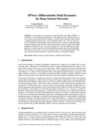
find the direction to the surface of the object. Without loss of generality, we describe how to do thisin 3D, but this method is applicable to any dimensionality. We construct ConvSDFX , which uses a3 1 1 kernel, i.e., 3 kernel cells all placed in a line along the X-axis. We set the kernel cell weightswk to -1 for the cell towards the negative X-axis, 1 for the cell towards the positive X-axis, and 0for the center cell. We construct ConvSDFY and ConvSDFZ similarly for the Y and Z axes. Byconvolving each of these 3 layers, we use local differencing in each of the X, Y, and Z dimensionsto compute the normal of the surface of the object nSDF , i.e., the direction to “push” the particle in.We can then update the particle positions P 0 as followsP 0 P 0 R nSDF .That is, we multiply the distance each particle is penetrating an object (R) by the direction to moveit in (nSDF ) and add that to the particle positions.Smooth Particle Networks (SPNets)5(a) Ladle SceneCohesion DifferenceCohesion 06050100150200IterationViscosity Difference50403020100-10Ground Truthλc , λv0.05, 300.05, 600.05, 900.10, 300.10, 600.10, 900.15, 300.15, 600.15, rationViscosity Difference504030DifferenceDifferenceUsing the ConvSP and ConvSDF layers described in the previous sectionsand standard network layers, we designSPNets to exactly replicate the PBF algorithm in figure 1. That is, at eachtimestep, the network takes in the current particle positions P and velocitiesV and computes the fluid dynamics byapplying the algorithm line-by-line, resulting in new positions P 0 and velocities V 0 . We show an SPNet layout diagram in the appendix. By repeatedlyapplying the network to the new positions and velocities at each timestep,we can simulate the flow of liquid overtime. We utilize elementwise layers,rectified linear layers (ReLU), and ourtwo particle layers ConvSP and ConvSDF to compute each line in figure 1.Since elementwise and ReLU layers aredifferentiable, and because we implement analytical gradients for ConvSPand ConvSDF, we can use backpropagation through the whole network to compute the gradients. Additionally, ourlayers are implemented with graphicsprocessor support, which means that aforward pass through our network takes1approximately 15of a second for about9,000 particles running on an Nvidia Titan Xp graphics ration(b) L1-Loss200050100150200250Iteration(c) Projection-LossFigure 2: (Top) The ladle scene. The left two images are beforeand after snapshots, the right image shows the particles projected onto a virtual camera image (with the objects shown indark gray for reference). (Bottom) The difference between theestimated and ground truth fluid parameter values for cohesionλc and viscosity λv after each iteration of training for both theL1 loss and the projection loss. The color of the lines indicatesthe ground truth λc and λv values.Evaluation & ResultsTo demonstrate the utility of SPNets, we evaluated it on three types of tasks, described in the following sections. First, we show how our model can learn fluid parameters from data. Next, we showhow we can use the analytical gradients of our model to do liquid control. Finally, we show how wecan use SPNets to train a reinforcement learning policy to solve a liquid manipulation task using policy gradients. Additionally, we also show preliminary results combining SPNets with convolutionalneural networks for perception.5
5.1Learning Fluid ParametersWe evaluate SPNets on the task of learning, or estimating, some of the λ fluid parameters from data.This experiment illustrates how one can perform system identification on liquids using gradientbased optimization. Here we frame this system identification problem as a learning problem so thatwe can apply learning techniques to discover the parameters. We use a commercial fluid simulatorto generate the data and then use backpropagation to estimate the fluid parameters. We refer thereader to the appendix for more details on this process.We used the ladle scene shown in Figure 2a to test our method. Here, the liquid rests in a rectangularcontainer as a ladle scoops some liquid from the container and then pours it back into the container.Figures 2b and 2c show the difference between the ground truth and estimated values for the cohesion λc and viscosity λv parameters when using the model to estimate the parameters on each of the9 sequences we generated, for both the L1-loss, which assumes full knowledge of the particle state,and the projection loss, which assumes the system has access to only a 2D projection of the particlestate. In all 9 cases and for both losses, the network converges to the ground truth parameter valuesafter only a couple hundred iterations. While the L1 loss tended to converge slightly faster (which isto be expected with a more dense loss signal), the projection loss was equally able to converge to thecorrect parameter values, indicating that the gradients computed by our model through the cameraprojection are able to correctly capture the changes in the liquid due to its parameters. Note that forthe projection loss the camera position is important to provide the silhouette information necessaryto infer the liquid parameters.5.2Liquid ControlTo test the efficacy of the gradients produced by our models, we evaluate SPNets on 3 liquid control problems. Thegoal in each is to find the set of controlsU {ut } that minimize the costXL l(Pt , Vt , ut )(4)twhere l is the cost function, Pt is the setof particle positions at time t, and Vt isthe set of particle velocities at time t.(a) Plate(b) Pouring(c) CatchingTo optimize the controls U, we utilizeModel Predictive Control (MPC) [38].MPC optimizes the controls for a short, Figure 3: The control scenes used in the evaluations in thispaper. The top row shows the initial scene; the bottom rowfinite time horizon, and then re-optimizes shows the scene after several seconds.at every timestep. We evaluated ourmodel on 3 scenes: the plate scene, the pouring scene, and the catching scene. We refer the readerto the appendix for details on how MPC is used to optimize the controls for each scene.The Plate Scene: Figure 5a shows the plate scene. It consists of a plate surrounded by 8 bowls.A small amount of liquid is placed on the center of the plate, and the plate must be tilted such thatthe liquid falls into a given target bowl. Figure 4a shows the results of each of the evaluations onthe plate scene. In every case, the optimization produced a trajectory where the plate would “dip”in the direction of the target bowl, wait until the liquid had gained sufficient momentum, and thenreturn upright, which allowed the liquid to travel further off the edge of the plate. Note that simply“dipping” the plate would result in the liquid falling short of the bowl. For all bowls except one, thisresulted in 100% of the liquid being placed into the correct bowl. For the one bowl, when it was setas the target, all but a small number of the liquid particles were placed in the bowl. Those particleslanded on the lip of the bowl, eventually rolling off onto the ground. Nonetheless, it is clear that ourmethod is able to effectively solve this task in the vast majority of cases.The Pouring Scene: We also evaluated our method on the pouring scene, shown in Figure 5b.The goal of this task is to pour liquid from the cup into the bowl. In all cases we evaluated, allliquid either remained in the cup or was poured into the bowl; no liquid was spilled on the ground.For that reason, in figure 4b we show how close each evaluation was to the given desired pouramount. In every case, the amount poured was within 11g of the desired amount, and the average6
0%100%Actual (g)100%200150100100%100150200250Target (g)(a) Plate olicyTest99.2%93.8%96.5%(c) Catching Scene(b) Pouring SceneFigure 4: Results from the liquid control task. From left to right: The plate scene. The numbers in each bowlindicate the percent of particles that were successfully placed in that bowl when that bowl was the target. Thepouring scene. The x axis is the targeted pour amount and the y axis is the amount of liquid that was actuallypoured where the red marks indicate each of the 11 pours. The catching scene. Shown is the percent of liquidcaught by the target cup where the rows indicate the initial direction of movement of the source.difference across all 11 runs between actual and desired was 5g. Note that the initial rotation ofthe cup happens implicitly; our loss function only specifies a desired target for the liquid, not anyexplicit motion. This shows that physical reasoning about fluids using our model enables solvingfine-grained reasoning tasks like this.The Catching Scene: The final scene we evaluated on was the catching scene, shown in Figure 5c.The scene consisted of two cups, a source cup in the air filled with liquid and a target cup on theground. The source cup moved arbitrarily while dumping the liquid in a stream. The goal of thisscene is to shift the target cup along the ground to catch the stream of liquid and prevent it fromhitting the ground. The first column of the table in Figure 4c shows the percentage of liquid caughtby the cup averaged across our evaluations. In all cases, the vast majority of the liquid was caught,with only a small amount dropped due largely to the time it took the target cup to initially moveunder the stream. It is clear from these results and the liquid control results on the previous twoscenes that our model can enable fine-grained reasoning about fluid dynamics.5.3Learning a Liquid Control Policy via Reinforcement LearningFinally, we evaluate our model on the task of learning a policy in a reinforcement learning setting.That is, the control ut at timestep t is computed as a function of the state of the environment, ratherthan optimized directly as in the previous section. Here the goal of the robot is to optimize theparameters of the policy. We refer the reader to the appendix for details on the policy trainingprocedure. We test our methodology on the catching scene. The middle column of the table infigure 5c shows the percent of liquid caught by the target cup when using the policy to generate thecontrols for the training sequences. In all cases, the vast majority of the liquid was caught by thetarget cup. To test the generalization ability of the policy, we modified the sequences as follows. Forall the training sequences, the source cup rotated counter-clockwise (CCW) when pouring. To testthe policy, we had the source cup follow the same movement trajectory, but rotated clockwise (CW)instead, i.e., in training the liquid always poured from the left side of the source, but for testing itpoured out of the right side. The percent of liquid caught by the target cup when using the policyfor the CW case is shown in the third column of the table in figure 5c. Once again the policy is ableto catch the vast majority of the liquid. The main point of failure is when the source cup initiallymoves to the left. In this case, as the source cup rotates, the liquid initially only appears in theupper-left of the image. It’s not until the liquid has traveled downward several centimeters that thepolicy begins to move the target cup under the stream, causing it to fail to catch the initial liquid.This behavior makes sense, given that during training the policy only ever encountered the sourcecup rotating CCW, resulting in liquid never appearing in the upper-left of the image. Nonetheless,these results show that, at least in this case, our method enables us to train robust policies for solvingliquid control tasks.5.4Combining SPNets with PerceptionWhile the focus in this paper has been on introducing SPNets as a platform for differentiable fluiddynamics, we also wish to show an example of how it can be combined with real perception. So inthis section we show some initial results on a liquid state tracking task. That is, we use a real robotand have it interact with liquid. During the interaction, the robot observes the liquid via its camera.7
It is then tasked with reconstructing the full 3D state of the liquid at each point in time from thisobservation. To make this task feasible, we assume that the initial state of the liquid is known andthat the robot has 3D models of and can track the 3D pose of the rigid objects in the scene. Therobot then uses SPNets to compute the updated liquid position at each point in time, and uses theobservation to correct the liquid state when the dynamics of the simulated and real liquid begin todiverge. This is the same task we looked at in [21]. We describe the details of this method in theappendix.We evaluated the robot on 12 pouringsequences. Figure 5 shows 2 exampleframes from 2 different sequences andthe result of both SPNets and SPNetswith perception. The yellow pixels indicate where the model and ground truthagree; the blue and green where they disagree. From this it is apparent that SPNets with perception is significantly better at matching the real liquid state thanSPNets without perception. We evaluate the intersection-over-union (IOU)across all frames of the 12 pouring sequences. SPNets alone (without perception) achieved an IOU of 36.1%. SPNets with perception achieved an IOU(a) RGB(b) SPNets(c) SPNets Perceptionof 56.8%. These results clearly showthat perception is capable of greatly im- Figure 5: Results when combining SPNets with perception.proving performance even when there is The images in the top and bottom rows show 2 example frames.significant model mismatch. Here we From left-to-right: the RGB image (for reference), the RGBcan see that SPNets with perception in- image with SPNets overlayed (not using perception), and thecreased performance by 20%, and from RGB image with SPNets with perception overlayed. In thethe images in Figure 5 it is clear that overlays, the blue color indicates ground truth liquid pixels,this increase in performance is signifi- green indicates the liquid particles,
new layers to the neural network toolbox: ConvSP and ConvSDF, which enable computing physical interactions with unordered particle sets. We use these lay-ers in combination with standard neural network layers to directly implement fluid dynamics inside a deep network, where th