WIXLIB

I-2.3 The unit level causal effects cannot be observed; remember the fundamental problem of causal inference. Thatmeans that population level causal effects also cannot be observed, even under SUTVA. To learn about causal effects, we must have replication. In the example above, we require some units withYi (Asp) observed and some with Yi (Not) observed. The assignment mechanism determines how to choose which potential outcome we will observe for each unit.Formally, the assignment mechanism is a probabilistic or deterministic rule for selecting some units to receivecontrol and other units to receive treatment. It describes what we do (or what was done) to learn about thescience: X, Y(1), Y(0). The assignment mechanism is critical, even if SUTVA holds. We must know or posit a rule for how each unitreceived treatment or control.8

I-3.1Subsection 3: Transition to Statistical Inference: The Perfect Doctor And Lord’s ParadoxDefinition of Basic ConceptsIgnorable Assignment Mechanism: The assignment of treatment or control for all units is independent of theunobserved potential outcomes (“nonignorable” means not ignorable)Unconfounded Assignment Mechanism: The assignment of treatment or control for all units is independent of allpotential outcomes, observed or unobserved (“confounded” means not unconfounded)Example I-7: Perfect DoctorThis example illustrates that we must consider the assignment mechanism to reach reliable causal inferences.The hypothetical data given below shows all potential outcomes under two different treatments: Y (0) representsyears lived after standard surgery and Y (1) represents years lived after new surgery.The “Truth”:Potential he true average causal effect Y (1) Y (0) 2.**Note: Y denotes Average of Y.The perfect doctor chooses the best treatment for each patient, i.e., the treatment under which the patient will livelonger. If there is no difference, he chooses by flipping a coin.9

I-3.2What we would actually observe under the Perfect Doctor’s assignment 14?1095.411Observed y1 y0 5.6 6 2.W indicates which treatment each unit received.In the perfect doctor example, the treatment each unit receives depends on that unit’s potential outcomes. Theassignment mechanism is nonignorable (and thus confounded). It is difficult to analyze correctly an experiment witha nonignorable assignment mechanism.For example, if we were to draw an inference based on the observed difference in sample means, we would concludethat the treatment, on average, adds over five years of life. But we “know” that the treatment, on average, subtractstwo years from life. Also, from looking at the observed sample means, we would conclude that if everyone receivedthe new operation, people would live an average of eleven years. But from the previous table, we “know” that ifeveryone received the new operation, people would live an average of five years. This is another incorrect inference.Moreover, from looking at all the observed values, we note that the years lived under the new operation (9, 10, 14)are much greater than the years lived under the old operation (4, 5, 6, 6, 6), an observation that could very easilylead to another incorrect causal inference.What’s wrong with what we did? Where exactly was our mistake? To get a better idea of what’s going on, let’s takea look at what would be observed in ALL POSSIBLE assignments in this situation.10

I-3.3The Perfect Doctor, continued: All Possible 1100000111Averagey1 .5-2.90.5-0.1-2median(y1 ) - median(y0 311

I-3.4As the chart on the previous page shows, there are 56 possible assignments in which three of eight units receivetreatment.Observed Outcomes underAssignment 56Observed Outcomes underAssignment 00000111ObservedAverages**Observed y1 y0 1.6.Y(0)136456?Y(1)?11096.86.7**Observed y1 y0 0.1.Summary of All 56 AssignmentsDifference inMedians (sd 3.21)0055101015201525Difference in Means(sd 3.12)-8-6-4-2024Difference in Means6-812-6-4-2024Difference in Medians6

I-3.5Our statistic was the difference in observed means, and on page I-3.3, we calculated the value of that statistic forall 56 possible assignments. The average of all of these possible values was -2, which equals exactly the “known”truth. This equality suggests that had our observed assignment been, say, a random draw of one of the 56 possibleassignments, we would have been OK on average (we will quantify exactly what we mean by “OK on average” insubsequent sections). Random draws do not depend on the potential outcomes, and thus the associated assignmentmechanism is unconfounded.In contrast, the Perfect Doctor’s assignment mechanism depended on the potential outcomes and was thereforenonignorable (implying that it was confounded). We observed with certainty the most extreme assignment possible,and the value of our statistic, the difference of observed sample means, was far from the truth; it even had the wrongsign. The difference of observed sample means is an OK estimate of the average causal effect, in general, only if theassignment mechanism is random.The takeaway message: The observed difference in means is entirely misleading in this situation. The biggestproblem when using the difference of sample means here is that we have effectively pretended that we had anunconfounded treatment assignment when in fact we did not. This example demonstrates the importance of findinga statistic that is appropriate for the actual assignment mechanism.13

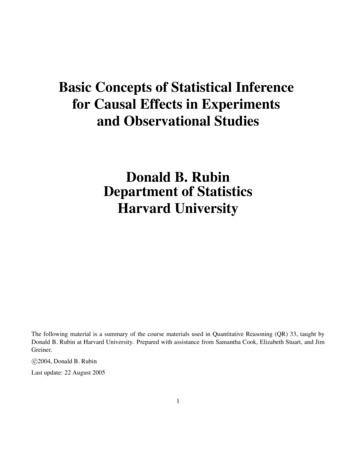
I-3.6Example I-8: Lord’s ParadoxFrom Holland and Rubin, “On Lord’s Paradox,” 1983.“A large university is interested in investigating the effects on the students of the diet provided in the universitydining halls and any sex differences in these effects. Various types of data are gathered. In particular, the weight ofeach student at the time of his [or her] arrival in September and his [or her] weight the following June are recorded.”% of Men0.20.50.71.72.58.010.015.415.014.814.017.2% of le averageJune weight114120122134146152158166176184191204Female averageJune weight102108110122134140146154164172179192Male Weight Gain Female Weight Gain121212121212121212121212250Weight for Males and FemalesMMMMMMMMMM MMMMMMMMMM MMMMMMMMMM MMM M M MM MM MMM MMM MMMMM MMMMM MMMMMM MMMFMMMFMMMalesMMMMMMMMMM M MMMMMMMMF MMMFMMMM MMMMFemalesMMMMMMMMMMMMMMMMMFM MMMMFMMMMMMMMMFFMMMMMM MMMM FMMFMMMMMMFMMMMMMMMMMMMMMMMMMMMFMMM MM MMMMFMFMMMMMMFMMMMMMMMMMMMMMMMFMMFF FFFMMMMFFFMMMMMMMFMFFFMFM MMFFM MMFMFFMMMMMMMMF FMMFMFMMMMMMMMMMMMMFMFMMMMMMMMMFMMMMMFFFMF M MFFFFMMMFMMFMMF FFFFFMMMFFFFMFFFMFFF M MMF MMFFMFFF MF FFMMMFFMMFMMMF FFMMFMF MFFFFFFFMFF MF FMFMFFFMFMFFFFMFFFF FFMFFFFFFFMMFFFFFFFMFMFFFFMFMFFF FFMFFFFFMFF MFF FFMMMFFFFMFFFMMFM MF FFFMFMFFFMFFFFFMFMMFFMFFMFFFFFMFFMFFFFFFMF FFFFFFFFFF FFFFFFFFFFFFFFFMFMFFMFFFFFFFFFFFFF MMMFFFFFFFMFFM FFF FF F FFFFFFF FFFFFFFFFFFFFMFFFFFMFFFFFFFFMFFFFFFMFFFFFFF FFFFMFM F FFFFFFFFFMFFFFMFFMFFF MF FF FFFFFFFFF F F FFF FFFFFFFFFFFFFFFFFFFF FFFF FF F FFFFFFFF F F FFFFF F FF FFFFF F FF FFF FFF FFFFFF F FFF FFF100150200250Weight in SeptemberMWeight in June150200M100Septemberweight range(in pounds) 69170-179180-189190-199 20014

I-3.7The average weight for Males was 180 in both September and June. Thus, the average weight gain for Males waszero.The average weight for Females was 130 in both September and June. Thus, the average weight gain for Femaleswas zero.Question: What is the differential causal effect of the diet on male weights and on female weights?Statistician 1: Look at gain scores: No effect of diet on weight for either males or females, and no evidence ofdifferential effect of the two sexes, because no group shows any systematic change.Statistician 2: Compare June weight (see Figure 1) for males and females with the same weight in September: Onaverage, for a given September weight, men weigh more in June than women. Thus, the new diet leads to moreweight gain for men.Is Statistician 1 correct? Statistician 2? Neither? Both?15

I-3.8Lord’s Paradox: Analysis under the Rubin Causal Model1. What are the units? The students, both male and female, in September.2. What are the treatments? The university dining hall diet, and the control diet, which is what the students wouldhave had otherwise.3. What is the assignment mechanism? Because all students in the study were exposed to the dining hall diet,the assignment mechanism is that all units receive treatment with probability one, and all units receive controlwith probability zero.4. Is the assignment mechanism unconfounded? Yes; for each unit, the probability of receiving treatment isunrelated to the potential outcomes.We can represent the Lord’s Paradox situation with the following table. The X’s, the covariates, are Sex andSep. Wt.Unit #12.nFnF 1nF 2.NSexFFSep. 81?240Here, Y(0), the outcome under control, represents what we would observe for a student had that student NOTeaten the dining hall diet. Because all students ate the dining hall diet, we observe this outcome for none ofthe units. Symbolically, p(Wi 1 Xi ) 1 for all i 1 to n. That is, the probability that we observe Y(1) isone for each unit.5. Is this assignment mechanism useful for causal inference? No; we observe the treated outcome for all unitsand the control outcome for none. To be useful for causal inference, the assignment mechanism must involvesome replication of each treatment.6. Would it have helped if all males received the dining hall diet and all females received the control diet? Notreally. We want replication at each value of X. That is, for each possible value of X we would like to see sometreated and some control units. The only way to achieve this result, even just in expectation, is to have randomassignment at each value of X.So, is Statistician 1 or Statistician 2 correct? In fact, we could make either one correct, depending on how we filledin Y(0) for each unit. Suppose we wanted to make correct Statistician 1’s assertion that there is no effect of treatmentfor men or for women. We could fill in each unit’s Y(0) value with its September weight. (Actually, we could alsofill in each unit’s Y(0) value with its June weight.) How implausible would these filled in Y(0) values be? We haveno idea from the observed data, because we did not observe Y(0) for any of the units.16

I-3.9Now suppose we wanted to make Statistician 2’s assertion that the new diet leads to more weight gain for mencorrect. For each male unit, we could predict Y(0) to be a constant plus that unit’s September weight times anotherconstant. We would have to choose the constants correctly (technically, they must come from the linear regressionof Y(1) on a vector of ones and September weight). We could do the same thing for each female unit. If wefollowed these steps, which would result in filling in a Y(0) value for each unit, Statistician 2 would be correct. Howimplausible would these Y(0) values be? We have no idea based on the observed data, because we did not observeY(0) for any of the units.The takeaway message: Both statisticians can be made correct even though they make contradictory assertions, andthus neither is correct, as the positions are stated. The key point is that everyone in this dataset received the treatment (the diet in the university dining halls). We observed Y(1) for all units and Y(0) for none. Would you want toassess the causal effect of a pill by giving everyone the pill? This dataset has no information in it about the effectof the dining hall diet on weight gain. To draw causal, rather than descriptive, inferences without making heroicassumptions, we need 0 p(Wi 1 Xi ) 1 for each unit! That is, we need not only an unconfounded assignment mechanism but also a stochastic (meaning probabilistic) assignment mechanism. A stochastic unconfoundedassignment mechanism is the most general form of a classical randomized experiment.17

I-4.1Subsection 4: Examples of Unconfounded Assignment Mechanisms, SimpleDefinition of Basic ConceptsPropensity Score: For each unit, the probability of being assigned treatment: p(Wi 1 X, Y (0), Y (1))Classical Randomized Assignment Mechanism: A special case of an unconfounded assignment mechanismwhere each unit’s assignment is probabilistic, i.e., the propensity score for each unit is strictly between 0 and 1Completely Randomized Assignment Mechanism: A special case of a randomized assignment mechanismwhere n of N units receive treatment, N - n (i.e., the rest) receive control, with each such assignment equally likelyExample I-9: Completely Randomized Design with N 2 units, 1 Assigned TreatmentW1 , X1 , Y1 (0), Y1 (1)@@W2 , X2 , Y2 (0), Y2 (1)@R@Assignment Mechanismk W (W1 , W2 ) Prob of W(0, 0)0(0, 1)0.5(1, 0)0.5(1, 1)018

I-4.2Example I-10: Completely Randomized Design with N 8 Units, 3 Assigned TreatmentW4 , X4 , Y4 (0), Y4 (1)W8 , X8 , Y8 (0), Y8 (1)W3 , X3 , Y3 (0), Y3 (1)W1 , X1 , Y1 (0), Y1 (1)W7 , X7 , Y7 (0), Y7 (1)W5 , X5 , Y5 (0), Y5 (1)W2 , X2 , Y2 (0), Y2 (1)W6 , X6 , Y6 (0), Y6 (1)@@@R@Assignment Mechanismk abWP8If i 1 Wi 3 aPIf 8i 1 Wi 6 3Prob of W1 b560i.e., if exactly 3 of the Wi ’s equal 156 is the number of ways to choose 3 items from 8In this example, each person has probability 38 of receiving treatment (and probability 85 of receiving control). Thus,each person’s propensity score is 38 . Note: Subscripting of units is arbitrary (i.e, random), that is, nothing wouldchange if we called the “first” unit Unit 3, and the “second” unit Unit 7, etc. (so long as we kept Unit 3’s W value,its X value, its Y(0) value, and its Y(1) value together). Such a rearrangement is called a “permutation.”19

I-4.3Example I-11: Completely Randomized Design with N units, n Assigned TreatmentW4 , X4 , Y4 (0), Y4 (1)Wn , Xn , Yn (0), Yn (1)W30 , X30 , Y30 (0), Y30 (1)W1 , X1 , Y1 (0), Y1 (1).W12 , X12 , Y12 (0), Y12 (1)W6 , X6 , Y6 (0), Y6 (1)@@@R@Assignment Mechanismk a Nn WPNIf i 1 Wi nPIf Ni 1 Wi 6 nProb of Wa N 1n0is the number of ways to choose n items from NnIn this example, each person has probability Nof receiving treatment (and thus probability 1 ncontrol). Thus, each person’s propensity score is N.20nNof receiving

I-4.4Example I-12: “Bernoulli” (fair coin-tossing) Assignment, 4 unitsAssignment is random and independent across units; moreover, each individual has the same probability of receivingtreatment 1. In this example, this probability is .5, i.e., it is equally likely for each person to receive treatment 0 ortreatment 1. Thus, each person’s propensity score is .5. Remember that the overall assignment is the collection ofall of the individuals’ assignments: W (W1 , W2 , W3 , W4 ).Because each individual’s treatment status is assigned independently of the other individuals, the overall assignmentprobability is the product of the individual probabilities, that is, the product of the propensity scores.All Possible AssignmentsW(0, 0, 0, 0)(0, 0, 0, 1)(0, 0, 1, 0)(0, 0, 1, 1)(0, 1, 0, 0)(0, 1, 0, 1)(0, 1, 1, 0)(0, 1, 1, 1)(1, 0, 0, 0)(1, 0, 0, 1)(1, 0, 1, 0)(1, 0, 1, 1)(1, 1, 0, 0)(1, 1, 0, 1)(1, 1, 1, 0)(1, 1, 1, 1)Prob of 4(.5)4(.5)4(.5)4(.5)4(.5)4(.5)4Question: Are there some randomized assignments that are less effective than others with respect to learning aboutthe causal effect of treatment versus control? Hint: Remember Lord’s Paradox.Question: Are there some randomized assignment mechanisms that are less effective than others with respect tolearning about the causal effect of treatment versus control?21

I-4.5Example I-13: “Bernoulli” (biased coin-tossing) Assignment, 4 UnitsSame as Example I-12, except that now the probability of receiving treatment 1 for each individual is .4. Again,treatment is assigned independently for each individual. As with the previous example, each person has the samepropensity score, but here, that score is .4.All Possible AssignmentsW(0, 0, 0, 0)(0, 0, 0, 1)(0, 0, 1, 0)(0, 0, 1, 1)(0, 1, 0, 0)(0, 1, 0, 1)(0, 1, 1, 0)(0, 1, 1, 1)(1, 0, 0, 0)(1, 0, 0, 1)(1, 0, 1, 0)(1, 0, 1, 1)(1, 1, 0, 0)(1, 1, 0, 1)(1, 1, 1, 0)(1, 1, 1, 1)Prob of W(.6)4(.4)1 (.6)3(.4)1 (.6)3(.4)2 (.6)2(.4)1 (.6)3(.4)2 (.6)2(.4)2 (.6)2(.4)3 (.6)1(.4)1 (.6)3(.4)2 (.6)2(.4)2 (.6)2(.4)3 (.6)1(.4)2 (.6)2(.4)3 (.6)1(.4)3 (.6)1(.4)4Question: Again, are there some assignments that are less effective than others with respect to learning about thecausal effect of treatment versus control? Are these assignments more or less likely than in the previous example? Doyou have any advice concerning the choice of assignment mechanism for a researcher based on the simple examplesof assignment mechanisms given thus far?22

I-5.1Subsection 5: Examples of Unconfounded Assignment Mechanisms, with Covariates – BlockingDefinition of Basic ConceptsCovariate: A characteristic of a unit unaffected by treatment, such as baseline headache in the Perfect Doctorexample, or September weight in the Lord’s Paradox exampleBlock: A set of individuals grouped together based on some covariateExample I-14: Randomization within BlocksIn this case we consider two blocks: one comprising four males and another comprising four females. Two malesand two females are chosen completely at random to receive treatment 1. The other two males and two femalesreceive treatment 0.Females: Xi FWFProb of WF P84 1If i 5 Wi 22P8If i 5 Wi 6 20Males: Xi MWMP

11. Theory and practice of matched sampling – using propensities and covariates III. Causal inference based on predictive distributions of potential outcomes 12. Predictive inference – intuition under ignorability 13. Matching to impute missing potential outcomes – donor pools 14. Fitting distinct pre