Transcription
CS229T/STAT231: Statistical Learning Theory (Winter 2016)Percy LiangLast updated Wed Apr 20 2016 01:36These lecture notes will be updated periodically as the course goes on. The Appendixdescribes the basic notation, definitions, and theorems.Contents1 Overview1.1 What is this course about? (Lecture 1)1.2 Asymptotics (Lecture 1) . . . . . . . .1.3 Uniform convergence (Lecture 1) . . .1.4 Kernel methods (Lecture 1) . . . . . .1.5 Online learning (Lecture 1) . . . . . . .2 Asymptotics2.1 Overview (Lecture 1) . . . . . . . . . . . . . . . . . . .2.2 Gaussian mean estimation (Lecture 1) . . . . . . . . .2.3 Multinomial estimation (Lecture 1) . . . . . . . . . . .2.4 Exponential families (Lecture 2) . . . . . . . . . . . . .2.5 Maximum entropy principle (Lecture 2) . . . . . . . . .2.6 Method of moments for latent-variable models (Lecture2.7 Fixed design linear regression (Lecture 3) . . . . . . . .2.8 General loss functions and random design (Lecture 4) .2.9 Regularized fixed design linear regression (Lecture 4) .2.10 Summary (Lecture 4) . . . . . . . . . . . . . . . . . . .2.11 References . . . . . . . . . . . . . . . . . . . . . . . . . . . . . .3). . . . . .3 Uniform convergence3.1 Overview (Lecture 5) . . . . . . . . . . . . . . . . . . . . .3.2 Formal setup (Lecture 5) . . . . . . . . . . . . . . . . . . .3.3 Realizable finite hypothesis classes (Lecture 5) . . . . . . .3.4 Generalization bounds via uniform convergence (Lecture 5)3.5 Concentration inequalities (Lecture 5) . . . . . . . . . . . .3.6 Finite hypothesis classes (Lecture 6) . . . . . . . . . . . .3.7 Concentration inequalities (continued) (Lecture 6) . . . . .3.8 Rademacher complexity (Lecture 6) . . . . . . . . . . . . .3.9 Finite hypothesis classes (Lecture 7) . . . . . . . . . . . .3.10 Shattering coefficient (Lecture 7) . . . . . . . . . . . . . 3667274
3.113.123.133.143.153.163.173.18VC dimension (Lecture 7) . . . . . . . . . . . .Norm-constrained hypothesis classes (Lecture 7)Covering numbers (metric entropy) (Lecture 8)Algorithmic stability (Lecture 9) . . . . . . . . .PAC-Bayesian bounds (Lecture 9) . . . . . . . .Interpretation of bounds (Lecture 9) . . . . . .Summary (Lecture 9) . . . . . . . . . . . . . . .References . . . . . . . . . . . . . . . . . . . . .4 Kernel methods4.1 Motivation (Lecture 10) . . . . . . . . . . . . . . . . . .4.2 Kernels: definition and examples (Lecture 10) . . . . . .4.3 Three views of kernel methods (Lecture 10) . . . . . . .4.4 Reproducing kernel Hilbert spaces (RKHS) (Lecture 10)4.5 Learning using kernels (Lecture 11) . . . . . . . . . . . .4.6 Fourier properties of shift-invariant kernels (Lecture 11) .4.7 Efficient computation (Lecture 12) . . . . . . . . . . . .4.8 Universality (skipped in class) . . . . . . . . . . . . . . .4.9 RKHS embedding of probability distributions (skipped in4.10 Summary (Lecture 12) . . . . . . . . . . . . . . . . . . .4.11 References . . . . . . . . . . . . . . . . . . . . . . . . . .76818896100104105107. . . . . . . . . . . . . . . . . . . . . . . . .class). . . . . . .1081091111141161211251311381391421425 Online learning5.1 Introduction (Lecture 13) . . . . . . . . . . . . . . . . . . . . .5.2 Warm-up (Lecture 13) . . . . . . . . . . . . . . . . . . . . . . .5.3 Online convex optimization (Lecture 13) . . . . . . . . . . . . .5.4 Follow the leader (FTL) (Lecture 13) . . . . . . . . . . . . . . .5.5 Follow the regularized leader (FTRL) (Lecture 14) . . . . . . . .5.6 Online subgradient descent (OGD) (Lecture 14) . . . . . . . . .5.7 Online mirror descent (OMD) (Lecture 14) . . . . . . . . . . . .5.8 Regret bounds with Bregman divergences (Lecture 15) . . . . .5.9 Strong convexity and smoothness (Lecture 15) . . . . . . . . . .5.10 Local norms (Lecture 15) . . . . . . . . . . . . . . . . . . . . . .5.11 Adaptive optimistic mirror descent (Lecture 16) . . . . . . . . .5.12 Online-to-batch conversion (Lecture 16) . . . . . . . . . . . . . .5.13 Adversarial bandits: expert advice (Lecture 16) . . . . . . . . .5.14 Adversarial bandits: online gradient descent (Lecture 16) . . . .5.15 Stochastic bandits: upper confidence bound (UCB) (Lecture 16)5.16 Stochastic bandits: Thompson sampling (Lecture 16) . . . . . .5.17 Summary (Lecture 16) . . . . . . . . . . . . . . . . . . . . . . .5.18 References . . . . . . . . . . . . . . . . . . . . . . . . . . . . . 911921932
6 Neural networks (skipped in class)6.1 Motivation (Lecture 16) . . . . . . . . . . . . . .6.2 Setup (Lecture 16) . . . . . . . . . . . . . . . . .6.3 Approximation error (universality) (Lecture 16) .6.4 Generalization bounds (Lecture 16) . . . . . . . .6.5 Approximation error for polynomials (Lecture 16)6.6 References . . . . . . . . . . . . . . . . . . . . . .1941941951961982002037 Conclusions and outlook7.1 Review (Lecture 18) . . . . . . . . . . . . . . . . . . . . . .7.2 Changes at test time (Lecture 18) . . . . . . . . . . . . . . .7.3 Alternative forms of supervision (Lecture 18) . . . . . . . . .7.4 Interaction between computation and statistics (Lecture 18).204204206208209A AppendixA.1 Notation . . . . .A.2 Linear algebra . . .A.3 Probability . . . .A.4 Functional analysis.211211212213215.3.
[begin lecture 1]1(1)Overview1.1What is this course about? (Lecture 1) Machine learning has become an indispensible part of many application areas, in bothscience (biology, neuroscience, psychology, astronomy, etc.) and engineering (naturallanguage processing, computer vision, robotics, etc.). But machine learning is not asingle approach; rather, it consists of a dazzling array of seemingly disparate frameworks and paradigms spanning classification, regression, clustering, matrix factorization, Bayesian networks, Markov random fields, etc. This course aims to uncover thecommon statistical principles underlying this diverse array of techniques. This class is about the theoretical analysis of learning algorithms. Many of the analysistechniques introduced in this class—which involve a beautiful blend of probability,linear algebra, and optimization—are worth studying in their own right and are usefuloutside machine learning. For example, we will provide generic tools to bound thesupremum of stochastic processes. We will show how to optimize an arbitrary sequenceof convex functions and do as well on average compared to an expert that sees all thefunctions in advance. Meanwhile, the practitioner of machine learning is hunkered down trying to get thingsto work. Suppose we want to build a classifier to predict the topic of a document (e.g.,sports, politics, technology, etc.). We train a logistic regression with bag-of-wordsfeatures and obtain 8% training error on 1000 training documents, test error is 13%on 1000 documents. There are many questions we could ask that could help us moveforward.– How reliable are these numbers? If we reshuffled the data, would we get the sameanswer?– How much should we expect the test error to change if we double the number ofexamples?– What if we double the number of features? What if our features or parametersare sparse?– What if we double the regularization? Maybe use L1 regularization?– Should we change the model and use an SVM with a polynomial kernel or a neuralnetwork?In this class, we develop tools to tackle some of these questions. Our goal isn’t togive precise quantitative answers (just like analyses of algorithms doesn’t tell you how4
exactly many hours a particular algorithm will run). Rather, the analyses will revealthe relevant quantities (e.g., dimension, regularization strength, number of trainingexamples), and reveal how they influence the final test error. While a deeper theoretical understanding can offer a new perspective and can aid introubleshooting existing algorithms, it can also suggest new algorithms which mighthave been non-obvious without the conceptual scaffolding that theory provides.– A famous example is boosting. The following question was posed by Kearnsand Valiant in the late 1980s: is it possible to combine weak classifiers (that get51% accuracy) into a strong classifier (that get 99% accuracy)? This theoreticalchallenge eventually led to the development of AdaBoost in the mid 1990s, asimple and practical algorithm with strong theoretical guarantees.– In a more recent example, Google’s latest 22-layer convolutional neural networkthat won the 2014 ImageNet Visual Recognition Challenge was initially inspiredby a theoretically-motivated algorithm for learning deep neural networks withsparsity structure.There is obviously a large gap between theory and practice; theory relies on assumptions can be simultaneously too strong (e.g., data are i.i.d.) and too weak (e.g., anydistribution). The philosophy of this class is that the the purpose of theory here not tochurn out formulas that you simply plug numbers into. Rather, theory should changethe way you think. This class is structured into four sections: asymptotics, uniform convergence, kernelmethods, and online learning. We will move from very strong assumptions (assumingthe data are Gaussian, in asymptotics) to very weak assumptions (assuming the datacan be generated by an adversary, in online learning). Kernel methods is a bit of anoutlier in this regard; it is more about representational power rather than statisticallearning.1.2Asymptotics (Lecture 1) The setting is thus: Given data drawn based on some unknown parameter vector θ ,we compute a parameter estimate θ̂ from the data. How close is θ̂ to θ ? For simple models such as Gaussian mean estimation and fixed design linear regression,we can compute θ̂ θ in closed form. For most models, e.g., logistic regression, we can’t. But we can appeal to asymptotics,a common tool used in statistics (van der Vaart, 1998). The basic idea is to take Taylorexpansions and show asymptotic normality: that is, the distribution of n(θ̂ θ )tends to a Gaussian as the number of examples n grows. The appeal of asymptotics isthat we can get this simple result even if θ̂ is very complicated!5
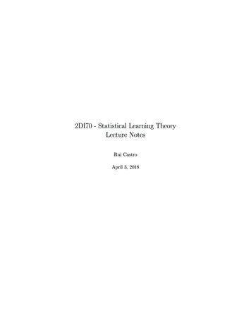
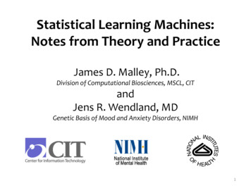
θ θ̂Figure 1: In asymptotic analysis, we study how a parameter estimate θ̂ behaves when itis close to the true parameters θ . Most of our analyses will be done with maximum likelihood estimators, which have nicestatistical properties (they have the smallest possible asymptotic variance out of allestimators). But maximum likelihood is computationally intractable for most latentvariable models and requires non-convex optimization. These optimization problemsare typically solved by EM, which is only guaranteed to converge to local optima. Wewill show how the method of moments, an old approach to parameter estimationdating back to Pearson (1894) can be brought to bear on this problem, yielding efficientalgorithms that produce globally optimal solutions (Anandkumar et al., 2012b).1.3Uniform convergence (Lecture 1) Asymptotics provides a nice first cut analysis, and is adequate for many scenarios, butit has two drawbacks:– It requires a smoothness assumption, which means you can’t analyze the hingeloss or L1 regularization.– It doesn’t tell you how large n has to be before the asymptotics kick in. Uniform convergence provides another perspective on the problem. To start, considerstandard supervised learning: given a training set of input-output (x, y) pairs, thelearning algorithm chooses a predictor h : X Y from a hypothesis class H and weevaluate it based on unseen test data. Here’s a simple question: how do the trainingerror L̂(h) and test error L(h) relate to each other? For a fixed h H, the training error L̂(h) is an average of i.i.d. random variables (losson each example), which converges to test error L(h) at a rate governed by Hoeffding’sinequality or the central limit theorem. But the point in learning is that we’re supposed to choose a hypothesis based on thetraining data, not simply used a fixed h. Specifically, consider the empirical risk6
expected risk Lempirical risk L̂h ĥERMFigure 2: We want to minimize the expected risk L to get h , but we can only minimizethe empirical risk L̂ to get ĥ.minimizer (ERM), which minimizes the training error:ĥERM arg min L̂(h).h H(1)Now what can we say about the relationship between L̂(ĥERM ) and L(ĥERM )? The keypoint is that ĥERM depends on L̂, so L̂(ĥERM ) is no longer an average of i.i.d. randomvariables; in fact, it’s quite a narly beast. Intuitively, the training error should besmaller than the test error and hence less reliable, but how do we formalize this?Using uniform convergence, we will show that:!rComplexity(H)L(ĥERM ) L̂(ĥERM ) Op.(2) {z } {z}ntest errortraining error The rate of convergence is governed by the complexity of H. We will devote a gooddeal of time computing the complexity of various function classes H. VC dimension,covering numbers, and Rademacher complexity are different ways of measuring how biga set of functions is. For example, we will see that if H contains d-dimensional linearclassifiers that are s-sparse, then Complexity(H) O(s log d), which means we cantolerate exponentially more irrelevant features! All of these results are distributionfree, makes no assumptions on the underlying data-generating distribution! These generalization bounds are in some sense the heart of statistical learning theory.But along the way, we will develop generally useful concentration inequalities whoseapplicability extends beyond machine learning (e.g., showing convergence of eigenvaluesin random matrix theory).7
1.4Kernel methods (Lecture 1) Let us take a detour away from analyzing the error of learning algorithms and thinkingmore about what models we should be learning. Real-world data is complex, so weneed expressive models. Kernels provide a rigorous mathematical framework to buildcomplex, non-linear models based on the machinery of linear models. For concreteness, suppose we’re trying to solve a regression task: predicting y Rfrom x X . The usual way of approaching machine learning is to define functions via a linearcombination of features: f (x) w · φ(x). Richer features yield richer functions:– φ(x) [1, x] yields linear functions– φ(x) [1, x, x2 ] yields quadratic functions Kernels provide another way to define functions. We define a positive semidefinite0kernel k(x, x0 ), which captures the “similarity” betweenPnx and x , and the define afunction by comparing with a set of exemplars: f (x) i 1 αi k(xi , x).– Kernels allow us to construct complex non-linear functions (e.g., Gaussian kernel0 k2)) that are universal, in that it can approximate anyk(x, x0 ) exp( kx x2σ 2continuous function.– For strings, trees, graphs, etc., can define kernels that exploit dynamic programming for efficient computation. Finally, we operate on the functions themselves, which is at the end of the day all thatmatters. We will define a space of functions called an reproducing kernel Hilbertspace (RKHS), which allows us to treat the functions like vectors and perform linearalgebra. It turns out that all three perspectives are getting at the same thing:Feature map φ(x)uniqueKernel k(x, x0 )Figure 3:uniqueRKHS H with k · kHThe three key mathematical concepts in kernel methods.8
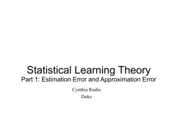
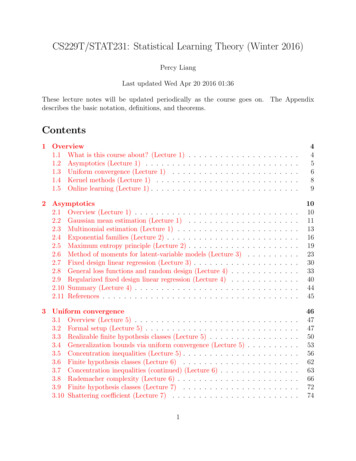
There are in fact many feature maps that yield the same kernel (and thus RKHS), soone can choose the one based on computational convenience. Kernel methods generallyrequire O(n2 ) time (n is the number of training points) to even compute the kernelmatrix. Approximations based on sampling offer efficient solutions. For example, bygenerating lots of random features of the form cos(ω · x b), we can approximate anyshift-invariant kernel. Random features also provides some intuition into why neuralnetworks work.1.5Online learning (Lecture 1) The world is a dynamic place, something that’s not captured well by our earlier analysesbased on asymptotics and uniform convergence. Online learning tries to do addressthis in two ways:– So far, in order to analyze the error of a learning algorithm, we had to assumethat the training examples were i.i.d. However in practice, data points mightbe dependent, and worse, they might be generated by an adversary (think spamclassification).– In addition, we have so far considered the batch learning setting, where we geta training set, learn a model, and then deploy that model. But in practice, datamight be arriving in a stream, and we might want to interleave learning andprediction. The online learning setting is a game between a learner and nature:x1p1y1Learner.NaturexTpTyTFigure 4: Online learning game.– Iterate t 1, . . . , T : Learner receives input xt X (e.g., system gets email)Learner outputs prediction pt Y (e.g., system labels email)Learner receives true label yt Y (e.g., user relabels email if necessary)(Learner updates model parameters)9
How do we evaluate?– Loss function: (yt , pt ) R (e.g., 1 if wrong, 0 if correct)– Let H be a set of fixed expert predictors (e.g., heuristic rules)– Regret: cumulative difference between learner’s loss and best fixed expert’s loss:in other words, how well did the learner do compared to if we had seen all thedata and chose the best single expert in advance? Our primary aim is to upper bound the regret. For example, for finite H, we will show:p(3)Regret O( T log H ).Things to note:– The average regretbest fixed expert).RegretTgoes to zero (in the long run, we’re doing as well as the– The bound only depends logarithmically on the number of experts, which meansthat the number of experts H can be exponentially larger than the number ofdata points T .– There is no probability here; the data is generated adversarially. What we relyon is the (possibly hidden) convexity in the problem. Online learning naturally leads to the multi-armed bandit setting, where the learneronly receives partial feedback. Suppose you’re trying to assign treatments pt to patientsxt . In this case, you only observe the outcome associated with treatment pt , not theother treatments you could have chosen (in the standard online learning setting, youreceive the true label and hence feedback about every possible output). Online learningtechniques can be adapted to work in the multi-armed bandit setting. Overall, online learning has many things going for it: it leads to many simple algorithms(online gradient descent) which are used heavily in practice. At the same time, thetheory is remarkably clean and results are quite tight.2Asymptotics2.1Overview (Lecture 1) Here’s the basic question: Suppose we have data points drawn from an unknowndistribution with parameters θ :x(1) , . . . , x(n) pθ .(4)Can we come up with an estimate θ̂ (some function of the data) that gets close to θ ?10
We begin with perhaps the simplest statistical problem: estimating the mean of a Gaussian distribution (Section 2.2). This allows us to introduce the concept of parametererror, and provides intuition for how this error scales with dimensionality and number of examples. We then consider estimating multinomial distributions (Section 2.3),where we get our first taste of asymptotics in order to cope with the non-Gaussianity,appealing to the central limit theorem and the continuous mapping theorem. Finally,we generalize to exponential families (Section 2.4), a hugely important class of models.Here, our parameter estimate is no longer an empirical average, so we lean on the deltamethod. We then introduce the method of moments, and show an equivalence with exponentialfamilies via the maximum entropy principle (Section 2.5). But the real benefit ofmethod of moments is in latent-variable models (Section 2.6). Here, we show thatwe can obtain an efficient estimator for three-view mixture models when maximumlikelihood would otherwise require non-convex optimization. Next, we turn from parameter estimation to prediction, starting with fixed design linearregression (Section 2.7). The analysis is largely similar to mean estimation, and we getexact closed form expressions. For the random design setting and general loss functions(to handle logistic regression), we need to again appeal to asymptotics (Section 2.8). So far, we’ve only considered unregularized estimators, which make sense when thenumber of data points is large relative to the model complexity. Otherwise, regularization is necessary to prevent overfitting. As a first attempt to study regularization,we analyze the regularized least squares estimator (ridge regression) for fixed designlinear regression, and show how to tune the regularization strength to balance thebias-variance tradeoff (Section 2.9).2.2Gaussian mean estimation (Lecture 1) We warmup with a simple classic example from statistics. The goal is to estimate themean of a Gaussian distribution. Suppose we have n i.i.d. samples from a Gaussiandistribution with unknown mean θ Rd and known variance σ 2 I (so that each of thed components are independent):x(1) , . . . , x(n) N (θ , σ 2 I)(5) Define θ̂ to be parameter estimate equal to the sample mean:nθ̂ 1 X (i)x .n i 1(6) Let us study how this estimate θ̂ deviates from the true parameter θ:θ̂ θ Rd .11(7)
This deviation is a random vector which should depend on the number of points n andthe variance σ 2 . What do you think the dependence will be? Lemma 1 (parameter deviation for Gaussian mean)– The sample mean estimate θ̂ deviates from the true parameter θ according to aGaussian: σ2I .(8)θ̂ θ N 0,n– FIGURE: [θ̂ in a ball around θ for d 2] Proof of Lemma 1– We need the following basic properties of Gaussians: Fact 1 (sums of independent Gaussians): if v1 N (0, Σ1 ) and v2 N (0, Σ2 )are independent, then v1 v2 N (0, Σ1 Σ2 ). Fact 2 (constant times Gaussian): if v N (0, Σ), then Av N (0, AΣA )for any matrix A.– The rest is just algebra: First, note that x(i) θ N (0, σ 2 I).def P Next, we have that Sn ni 1 x(i) N (0, nσ 2 I) by Fact 1. 2 Finally, we have θ̂ θ Snn N 0, σnI by Fact 2. Lemma 1 tells us how the entire estimated vector behaves, but sometimes it’s convenient to just get one number that tells us how we’re doing. Let’s define the meansquared parameter error, which is the squared distance between the estimate θ̂ andthe true parameter θ :kθ̂ θ k22 .(9)How do you think the parameter error behaves? Lemma 2 (parameter error for Gaussian mean)– The mean-squared parameter error is:kθ̂ θ k22 σ2 2χ ,n d(10)and has expected value:hi dσ 2E kθ̂ θk22 .n12(11)
Proof of Lemma 2– Standard properties of chi-squared distributions:P If v1 , . . . , vd N (0, 1), then dj 1 vj2 χ2d . If z χ2d , then E[z] d and Var[z] 2d.p– By Lemma 1, we know that v σn2 (θ̂ θ ) N (0, I).P– The squared 2-norm of this vector (kvk22 dj 1 vj2 ) is therefore distributed asχ2d .– Multiplying both sides byσ2nyields (10).– Taking expectations on both sides yields (11). A Gaussian random vector has fluctuations on the orderqof its standard deviation, we2can think of θ̂ having typical deviations on the order of dσn . FIGURE: [relate to previous figure, density of a chi-squared for kθ̂ θ k22 ] Takeaways– Life is easy when everything’s Gaussian, since we can compute things in closedform.– Think geometrically about shrinking balls around θ .2.3Multinomial estimation (Lecture 1) In the above, things worked out nicely because everything was Gaussian. What if aredata are not Gaussian? Suppose we have an unknown multinomialPd distribution over d choices: θ d (that is,θ [θ1 , . . . , θd ], θj 0 for each j and j 1 θj 1). Suppose we have n i.i.d. samplesfrom this unknown multinomial distributionx(1) , . . . , x(n) Multinomial(θ ),(12)where each x(i) {e1 , . . . , ed } and ej {0, 1}d is an indicator vector that is 1 atposition j and 0 elsewhere. Consider the empirical distribution as the estimator (same form as the sample mean):n1 X (i)θ̂ x .n i 1 Example:13(13)
– θ [0.2, 0.5, 0.3]– x(1) [0, 1, 0], x(2) [1, 0, 0], x(3) [0, 1, 0]– θ̂ [ 31 , 23 , 0] We can now ask the same question as we did for Gaussian estimation: what is theparameter error kθ̂ θ k22 ? Before we had gotten a chi-squared distribution becausewe had Gaussians and could work out everything in closed form. But now, we havemultinomial distributions, which makes things more difficult to analyze. How do youthink the parameter error will behave? Fortunately, not all hope is lost. Our strategy will be to study the asymptotic behavior of the estimators. By the central limit theorem, we have dn(θ̂ θ ) N (0, V ),(14)defwhere V diag(θ ) θ (θ ) is the the asymptotic variance of a single multinomialdraw. Written out, the elements of V are:(θj (1 θj ) if j k(15)Vjk if j 6 k. θj θk It is easy to check this by noticing that E[xj ] E[x2j ] θj , E[xj xk ] 0 for j 6 k.Further sanity check:– For a single component j, when θj is close to 0 or 1, the variance is small.– The covariance between components j and k is negative since the probabilitiessum to 1 (there is competition among components). Next, we can apply the continuous mapping theorem on the function k · k22 (seeAppendix), which lets us transfer convergence results through continuous functions:dnkθ̂ θ k22 tr(W(V, 1)),(16)where W(V, k) is the Wishart distribution (multivariate generalization of the chisquared) with mean matrix V and k degrees of freedom. This follows because z N (0, V ), then zz W(V, 1), and kzk22 tr(zz ).14
Taking expectations1 and dividing by n on both sides yields:! dhiX11 2 oE kθ̂ θ k2 θj (1 θj )nnj 1 11 o.nn(17)(18) Note that the n1 term is independent of d, unlike in the Gaussian case, where the result2was dσn . The difference is that in the Gaussian case, each dimension had standardq1deviation σ, whereas in the multinomial case here, it is aboutfor the uniformddistribution.d1This step actually requires additional justification. In particular, if we have Yn Y , in order toconclude E[Yn ] E[Y ], we need (Yn ) to be uniformly integrable. A sufficient condition is that Yn has finitesecond-order moments, which means that a data point needs to have finite fourth-order moments. This isclearly the case for the multinomial distribution (which is bounded), and will be true for exponential families(for which all moments exist), discussed in the next section. Showing this result formally is non-trivial andis out of the scope of this class.15
[begin lecture 2]2.4(2)Exponential families (Lecture 2) So far, we’ve analyzed the Gaussian and the multinomial. Now let us delve intoexponential families, a much more general family of distributions which include theGaussian, multinomial, gamma, beta, etc., but not things like the uniform distributionor mixture models. Exponential families are also the basis of undirected graphical models. You probablyfirst saw exponential families in a univariate continuous setting, but we will introducethem here in the multivariable discrete setting in order to build some different intuitions(and to simply the math). Definition 1 (exponential family)– Let X be a discrete set. Example: X { 1, 1}3– Let φ : X Rd be a feature function. Example (unary and binary factors):φ(x) [x1 , x2 , x3 , x1 x2 , x2 x3 ] R5 .(19)– Define a family of distributions P, where each pθ P assigns each x X aprobability that depends on x only through φ(x):defdefP {pθ : θ Rd },pθ (x) exp{θ · φ(x) A(θ)},(20)where the log-partition functiondefA(θ) logXexp{θ · φ(x)}(21)x Xensures the distribution is normalized.– Example: if θ [0, 0, 0, 0, 0], then pθ is the uniform distribution.– Example: if θ [0, 0, 0, log 2, 0] (which favors x1 and x2 having the same sign),then pθ assigns probability:16
x1 1 1 1 1 1 1 1 1x2 x3 1 1 1 1 1 1 1 1 1 1 1 1 1 1 1 1exp{θ · φ(x)}220.50.50.50.522pθ (x)0.20.20.050.050.050.050.20.2– Note that unlike multinomial distributions, P does not contain all possible distributions. Varying one parameter θj has the effect of moving all points x with thesame feature φ(x)j the same way.– FIGURE: [Venn diagram over outcome x, indicator features correspond to regions] A very useful property of exponential families is that derivatives of the log-partitionfunction correspond to moments of the distribution (a short algebra calculation thatyou should do once, but we’re going to skip):– The mean is the gradient of the log-partition function:Xdef A(θ) Eθ [φ(x)] pθ (x)φ(x).(22)x X– The covariance is the Hessian of the log-partition function:def 2 A(θ) Covθ [φ(x)] Eθ [(φ(x) Eθ [φ(x)])(φ(x) Eθ [φ(x)]) ].(23)– Note that since 2 A(θ) is a covariance matrix, it is necessarily positive semidefinite, which means that A is convex.– If 2 A(θ) 0, then A is strongly convex, and A is invertible (for intuition,consider the 1D case where A would be an increasing function). In this case,the exponential family is said to be minimal. For simplicity, we will assume weare working
Apr 20, 2016 · There is obviously a large gap between theory and practice; theory relies on assump-tions can be simultaneously too strong (e.g., data are i.i.d.) and too weak (e.g., any distribution). The philosophy of this class is that the the purpose of theory here not to churn out formulas that you simply plug nu