Transcription
Ground-Water HydraulicsGEOLOGICALSURVEY PROFESSIONAL PAPER708
Ground-Water HydraulicsBy S. W. LOHMANGEOLOGICAL SURVEY PROFESSIONAL PAPER 708UNITED STATES GOVERNMENT PRINTING OFFICE, WASHINGTON : 1972
UNITED STATES DEPARTMENT OF THE INTERIORROGERS C. B. MORTON, SecretaryGEOLOGICAL SURVEYV. E. McKelvey, DirectorFirst printing 1972Second printing 1975For sale by the Superintendent of Documents, U.S. Government Printing OfficeWashington, D.C. 20402 - Price 4.15 (paper cover)Stock Number 024-001-01194
CONTENTSPageSymbols and dimensions. --. .-.-. . . .Introduction---- .----- ---- ----- --------- .Divisions of subsurface water in unconfined aquifersSaturated zone.- --- - - --- --- - --Water table. . .Capillary fringe .- --------- ----.-.--. .Unsaturated --.----.----------.Hydrologic properties of water-bearing materials. -. .Porosity .Primary.- . . . - -. -------------- - .Secondary -------- ---- -.---------. -.Conditions controlling porosity of granular materials. . .Arrangement of grains (assumed spherical and ofequal size)--- -.--. .- .-.-.-- .----. .Shape of grains--------- -- --------- --- Degree of assortment.- -----. .Void ratio .------------ .--.-.-- . . .Permeabili ty -.----------- --------- - -Intrinsic permeability---.------ -----.--. .Hydraulic conductivity. . .Transmissivity . . . . .- -- ----. . .Water yielding and retaining capacity of unconfined aquifers.Specific yield.------------.--------------.-. .,Specific retention. - - - ---,-- -- .Moisture equivalent-Artesian wells confined aquifers ------- .Flowing wells unconfined aquifers . .Confined aquifers . .Potentiometric surface ------- --- -- - - Storage properties.-- -- -- -- ----- --- - .Storage coefficient .-- ---. . .-.-.Components - -.---.----. .Land subsidence. -.- . -.------.- . . .Elastic confined aquifers.- - --Nonelastic confined aquifers and oil-bearingstrata - - ---- -.-----Movement of ground water steady-state flow . . .Darcy's law. ------ -- - - -Velocity -- ---- ---- -.- . . .Aquifer tests by well methods point sink or point source.Steady radial flow without vertical movement.Example. ----- - -Partial differential equations for radial flow.Nonsteady radial flow without vertical movement.Constant discharge.- -. . . .Example. --- -- -- - -. .Straight-line solutions.TransmissivityStorage coefficient .----. . 889999101010111112131515191919212222Aquifer tests by well methods ContinuedNonsteady radial flow without vertical movementContinuedConstant drawdown . - ----Straight-line solutions---.Example . . .Instantaneous discharge or recharge"Slug" method. - . -- ---- -Example. - .----.--- ---.- . - .Bailer method- . .---------------------Leaky confined aquifers with vertical movement-.Constant discharge. . . - .--- . .Steady flow. ------ ----. .-.-- .Nonsteady flow. ------ ---Hantush-Jacob method. - --- - -----.Example. -- ---- . -------------.Hantusb modified method.-------------Example . . .Constant drawdown.-. .- .- -.- . .23232527272929303030303031323234Unconfined aquifers with vertical movement34Example for anisotropic aquifer.-. --. --- . .36Example for delayed yield from storage. .Aquifer tests by channel methods line sink or line source(nonsteady flow, no recharge). ---- ---.-.-----.---.Constant discharge .--- . . . -----.- - - .Constant drawdown.----------------.---------.---Aquifer tests by areal methods --. . .--------.Numerical analysis.------------ .-.-------------Example.--------.---- ----------------Flow-net analysis. ---.-.-- -.- .--.--- -----.--Example . - .------- -------------.-----.- Closed-contour method-- .--------------- ----- -.Unconfined wedge-shaped aquifer bounded by twostreams.-.-- ------------------- -------------Methods of estimating transmissivity . --- ---- .Specific capacity of wells---.---.-------------------Logs of wells and test holes. --.----------.---.Methods of estimating storage coefficient -- -- -- - Methods of estimating specific yield.-.-. -------- - .Drawdown interference from discharging wells. ---- --Relation of storage coefficient to spread of cone of depression.Aquifer boundaries and theory of images. - -- -- -"Impermeable" barrier. - - -- ------.Line source at constant head perennial streamApplication of image theory. . --- --- ."Safe yield". . .The source of water derived from wells- - -- --------- Examples of aquifers and their developmentValley of large perennial stream in humid region.Valley of ephemeral stream in semiarid region .Closed desert basin . . . .Southern High Plains of Texas and New MexicoGrand Junction artesian basin, Colorado. --References cited- . ------------- 3555657575859616264646465656667
IVCONTENTSILLUSTRATIONS[Plates are in pocket]PLATE 1. Logarithmic plot of a versus (?(«).2. Type curves for H/H0 versus Tt/rcz for five values of a;3.4.5.6.7.Two families of type curves for nonsteady radial flow in an infinite leaky artesian aquifer.Family of type curves for 1/u versus H(u, /3), for various values of j8.Logarithmic plot of a versus G(a, rw/B).Curves showing nondimensional response to pumping a fully penetrating well in an unconfined aquifer.Curves showing nondimensional response to pumping a well penetrating the bottom three-tenths, of the thickness of an unconfine.daquifer.8. Delayed-yield type curves.9. Logarithmic plot of SW(w) versus l/up.PageFIGURE 1. Diagram showing divisions of subsurface water in unconfined aquifers- - - --- - - - --. - . . .--- --.2-5. Sketches showing2. Water in the unsaturated zone ---- - --- - - -. - . . . . . .3. Capillary rise of water in a tube --------------- ---- - - - --- - - - - -- -- .-. .-. . .4. Rise of water in capillary tubes of different diameters . . . - - - . . . . . . . .5. Sections of four contiguous spheres of equal size . . -. - - -- - -- - --. . - . -. . .6. Graph showing relation between moisture equivalent and specific retention . - - . . . . . - .7. Diagrammatic section showing approximate flow pattern in uniformly permeable material which receives recharge ininterstream areas and from which water discharges into streams . .-- - --- - -8. Diagrammatic sections of discharging wells in a confined aquifer and an unconfined aquifer. . . . . .9. Sketch showing hypothetical example of steady flow10. Half the cross section of the cone of depression around a discharging well in an unconfined aquifer - . . . 11. Semilogarithmic plot of corrected drawdowns versus radial distance for aquifer test near Wichita, Kans 12. Sketch of cylindrical sections of a confined aquifer13. Sketch to illustrate partial differential equation for steady radial flow.-- - - - - -- - - - - - -.14. Logarithmic graph of W(u) versus u.15. Sketch showing relation of W(u) and u to s and r*/t, and displacements of graph scales by amounts of constants shown.16. Logarithmic plot of s versus r*/t from table 6 - - - - .- - - - ---- - - - -- ---17-19. Semilogarithmic plot of17. sw/Q versus t/rw2.,. . . . . . . . . . .-.18. Recovery (sw) versus t. . . . . . .19. Data from "slug" test on well at Dawsonville, Ga . . . . . . . . .20. Logarithmic plot of s versus t for observation well 23S/25E-17Q2 at Pixley, Calif . . . .21. Sketch showing relation of 2 to b of pumped and observation wells on plates 6 and 7.22-25. Logarithmic plot of22. s versus t for observation well B2-66-7dda2, near lone, Colo . .- . . . - --23. s versus t for observation well 139, near Fairborn, Ohio. -. .-. . . .-. . .- . . . - . - 24. D(u)q versus w2 for channel method constant discharge - - - - --- --- --- 25. D(u)h versus uz for channel method constant drawdown. . . . . -. . - - -.- .-- ---26. Sketch showing array of nodes used in finite-difference analysis ! . -.- - .-- - -.-- -.-. ----- .27. Plot of 2ft versus Aft0/AJ for winter of 1965-66, when W 0.28. Plot of 2A versus AAo/Af for spring-of 1966. . .,. ----------. . . .29. Sketch showing idealized square of flow net . ------------ -------------- -.------30. Map of Baltimore industrial area, Maryland, showing potentiometric surface in 1945 and generalized flow lines in thePatuxent Formation . .31. Sketch map of a surface drainage pattern, showing location of observation wells that penetrate an unconfined aquifer.32. Example hydrograph from well A of figure 31, showing observed and projected water-level altitudes .--.33. Graph of S/SQ versus t taken from hydrograph of well A (see fig. 32), showing computation of T/S. .34. Graph of s/s0 versus Tt/i*S for 00 75 ; 6/6a 0.20.35. Family of Semilogarithmic curves showing the drawdown produced at various distances from a well discharging at statedrates for 365 days from a confined aquifer for which T 20 ftzday-1 and S 5X 10 6 -- - - ---- - -----36. Family of Semilogarithmic curves showing the drawdown produced after various times at a distance of 1,000 ft from awell discharging at stated rates from a confined aquifer for which T 20 ft2day-1 and S 5X 10 5 ---- - -37. Idealized section views of a discharging well in an aquifer bounded by an "impermeable" barrier and of the equivalenthydraulic system in an infinite aquifer - --- - - -------38. Generalized flow net in the vicinity of discharging real and image wells near an "impermeable" boundary - - 39. Effect of "impermeable" barrier on Semilogarithmic plot of s versus i/r2 . - - - - - ---- ------40. Idealized section views of a discharging well in an aquifer bounded by a perennial stream and of the equivalent hydraulicsystem in an infinite aquifer . . . . . . . . . . - - ---- -- -------- 7474849505051545556575859
CONTENTSVPage41. Generalized flow net in the vicinity of a discharging well dependent upon induced infiltration from a nearby stream42. Effect of recharging stream on semilogarithmic plot of s versus t/r*. . . . . . . . . . . . . .43-47. Diagrammatic sections showing development of ground water from43. Valley of large perennial stream in humid region. . -. . . . . . . . . . . . . .44. Valley of ephemeral stream in semiarid region. . . . . . . . . . . . . .45. Bolson deposits in closed desert basin -.--. . - --- .-.-.- -. . . . . . . .46. Southern High Plains of Texas and New Mexico.- - - - -- ---- - -- - ---- - --- - - - - - .47. Grand Junction artesian basin, Colorado - - -- -- -- - - -- - - ------- - - --60616464656666TABLESTABLE 1.2.3.4.5.6.7.8.9.10.11.12-14.Capillary rise in samples having virtually the same porosity, 41 percent, after 72 days - . - - --- -. . .Relation of units of hydraulic conductivity, permeability, and trarismissivity . . . . . . . . .Land subsidence in California oil and water fields-------- -- ---- -- ----- --- -Data for pumping test near Wichita, Kans .Values of W(u) for values of u between 10 15 and 9.9---------- -------- - - - ---- - - - - - -Drawdown of water level in observation wells N-l, N-2, and N-3 at distance r from well being pumped at constant rateof 96,000 ft8 day-1.--.--.-.Values of G(a) for values of a between 10"* and 1015 -- - - . .Field data for flow test on Artesia Heights well near Grand Junction, Colo., September 22, 1948- - - -- - -Field data for recovery test on Artesia Heights well near Grand Junction, Colo., September 22, 1948. -, -- -Recovery of water level in well near Dawsonville, Ga., after instantaneous withdrawal of weighted float . -.-Postulated water-level drawdowns in three observation wells during a hypothetical test of ah infinite leaky confined aquifer.Drawdown of water levels inPage3510121619242426293112. Observation well 23S/25E-17Q2, 1,400 ft from a well pumping at constant rate of 750 gpm, at Pixley, Calif.,15.16.17.18.19.March 13, 1963.13. Observation well B2-66-7dda2, 63.0 ft from a well pumping at average rate of 1,170 gpm, near lone, Coio.,August 15-18, 1967. .14. Observation well 139, 73 ft from a well pumping at constant rate of 1,080 gpm, near Fairborn, Ohio, October19-21, 1954 . . . . .IValues of D(u) ,, u, and u2 for channel method constant discharge.------------ - - . . -Values of D(u\ u, and u? for channel method constant drawdownAverage values of hydraulic conductivity of alluvial materials in the Arkansas River valley, Colorado -. -.-Computations of drawdowns produced at various distances from a well discharging at stated rates for 365 days from aconfined aquifer for which T 20 ft2 day-1 and S 5X10⁻⁶.-. . . . .Computations of drawdowns produced after various times at a distance of 1,000 ft from a well discharging at stated ratesfrom a confined aquifer for which T 20 ft2 day-1 and S 5X10"5----- . . .3238384143535455
Symbol[Number in parentheses refers to the equation, page, or illustration where thesymbol first appears or where additional clarification may be obtained. Symbolsare also defined in the text. There is some duplication of symbols because of thedesire to preserve the notation used in the original papers]SymbolDimmtiontL*ABBBBECC,C'L*DD(u),E.r/a, Tt/r*S)HJJo, Jt(x)KKK', K"KrK,Li, LiL(u,v)MVIDetcriptionArea (8) ; area of influence (145) .l/VT/(K'/V) (95).(107).Constant (140).Barometric efficiency of artesianwell (22).Constant (7).Constant of proportionality (144).Discharge rate per unit area (151).D (drain) function of u for constantdischarge (112).D (drain) function of u for constantdrawdown (118).Bulk modulus of elasticity of solidskeleton of aquifer (20) .Bulk modulus of elasticity of water(20).F function of 80, O/Oo, r/a, Tt/r*S(p. 49).G function of a (68).G function of a, rv/B (96).Head inside well at time t afterinjection or removal of "slug"(75).Head inside well at instant ofinjection or removal of "slug"(75).H function of u, ft (91).Joule (9).Bessel function of zero order, firstkind (68), (100).Bessel function of first order, firstkind (75).Hydraulic conductivity (13), (92).Average hydraulic conductivity (p.H).Constant n/rp (150).Vertical hydraulic conductivity ofconfining beds (86), (92).Radial hydraulic conductivity (102) .Vertical hydraulic conductivity (102).Modified Bessel function of secondkind, zero order (96) .Modified Bessel function of secondkind, first order (96).Lengths of two concentric closedcontours (137).L (leakance) function of u, v (87).Moisture equivalent (18).Ratio: specific retention/moistureequivalent (18).DimmnontHT-i-- -.--.-M T * 471-1- .- L»LT l. .--- --- -Bessel function of zero order, secondL*T l 171-1SS'ML-i T-tLT l. . .----.---.-S', S"- - -- -S.St-.- ---. --.-.-- L }PRSrS., S.', S."TTTEVWW(u)DescriptionFlow rate (8); constant dischargerate (19); total flow (132).Constant discharge rate of drain perunit length of drain (112).Discharge of aquifer to drain perunit length of drain (120).Pressure (fig. 3).Recharge rate per unit area (151).Storage coefficient (19).Corrected value of storage coefficient (64).Storage coefficients of aquifer andsemipervious confining layers (92).Early time storage coefficient (107).Later time specific yield (107).Specific retention (17).Specific storage of aquifer and confining beds, respectively (92).Specific yield (16).Surface tension of fluid (1).Transmissivity (26), (19).Tidal efficiency of artesian well (22).Total volume (4).V function of and T (103).Rate of accretion (126).W (well) function of u (46).dkind (68).- ---.- Bessel function of first order, secondkind (77).LFinite length (128).LThickness of aquifer (p. 6).LThickness of confining bed (86).LCentimeter (p. 3), (11).LMTCentimeter-gram-second (11).LMean grain diameter (7).Derivative (8).e- - --- -ftQLLT *abVcmcgsdgalggpdgpmhJ* hi tohein.kkgBase of Naperian logarithms, 2.71828(p. 19).Foot (13).Standard acceleration due to gravity(8).UU.S. gallon (36).MGram.LT-1Gallons per day (p. 6).L*T lGallons per minute (p. 8).LHead (8), (116), (130).LHead at node (well) 0 (128), (129). Head at nodes (wells) 1 to 4 (fig.26), (128).LHeight of capillary rise (1).LInch (p. 9).L*Intrinsic permeability (7), (8).MKilogram (9).
VIISYMBOLS AND DIMENSIONSSymbolDimmriantLIlbmmmminnridnf-LLTLT lLLLLLsectTTL*SymbolDetentionLength of flow (8).Pound (p. 9).Meter (9).Millimeter (p. 3).Minute (36).S. St/S, (108).Number of potential drops (133) .Number of flow channels (132) .Rate of flow per unit area (specificdischarge) (8), (151).Radius or radial distance (1), (19).Radius of casing in interval overwhich water level fluctuates (76) .Radial distance from observationwell to image well (148).Radial distance from observationwell to pumped well (148).Radius of well screen or open hole(76).Radius of discharging well (67),(139).Drawdown (19), (114).Residual drawdown (81).Drawdown in image well (146).Abrupt change in drain level att 0 (118); abrupt change inwater level (fig. 32).Algebraic sum of sp and s (146).Drawdown in pumped well (146).Drawdown in discharging well (67),(139).Second (9).Time since discharge beganstopped (19).Variable of integration ( 19) ; r*»S/4 Tt(45), (85), (91);x\/is74T« (113).(r,-/rp)*Mp (149).tt,/(r /rp)» (149).Volume of water per unit time (37).(85), (86).Average velocity (28).Volume of water drained by gravity(16).Volume of interstices 'Volume of mineral particles (4).Volume of water retained againstgravity (17).L*Volume of water (4).LLength (130). . Variable of integration (68), (108).LDistance from drain to point ofobservation (112).LCoordinate in x direction (126).LCoordinate in y direction (126).Variable of integration (85), (91).LElevation head (99).LCoordinate in z direction (fig. 21). . Infinity (19). Summation (128). Angle (1); Tt/SrJ (67), (94);r.*S/rc» (76); (r/B)*/r*St (107).M-*LT*l/E. (21).M-iLT*l/E, (21). 2Vr.«(77) rjf [KM{&8?\4&VV K8. \ KS. ) (92) 'yAdML *T *Specific weight per unit area (20).-.--.-.-. Finite difference, change in (24). Partial derivative (37).(108).j eML l T lDynamic viscosity (10). Porosity (4); angle (138).0o.MX. Micro (10-«) (p. 5).---.-.-. Variable of integration (100).vL*T lKinematic viscosity (8), (10).r.3.1416.pPdML *ML lPmp«,T ?*Angle (138).Density of fluid (1).Density of dry sample (bulk density) (5).ML *Mean density of mineral particles(grain density) (5).ML *Density of water (18). Kt/Sb (100), (101); variable ofintegration (107).L*T *Potential (8). r/6 (100), (101).
GROUND-WATER HYDRAULICSBy S. W. LOHMANINTRODUCTIONThe science of ground-water hydrology is concerned withevaluating the occurrence, availability, and quality ofground water. Although many ground-water investigationsare qualitative in nature, quantitative studies are necessarily an integral part of the complete evaluation ofoccurrence and availability. The worth of an aquifer as asource-of water depends largely upon two iriherent characteristics its ability to store and to transmit water.Thorough knowledge of the geologic framework isessential to understand the operation of the naturalplumbing system within it. Ground-water hydraulics isconcerned with the natural or induced movement of waterthrough permeable rock formations. The principal methodof analysis in ground-water hydraulics is the application,generally by field tests of discharging wells, of equationsderived for particular boundary conditions. Prior to 1935,such equations were known only for the relatively simplesteady flow condition, which incidentally generally doesnot occur in nature. The development by Theis (1935), ofan equation for the nonsteady flow of ground water was amilestone in ground-water hydraulics. Since 1935 thenumber of equations and methods has grown rapidly andsteadily. These are described in a wide assortment ofpublications, some of which are not conveniently availableto many engaged in ground-water studies. The essence ofmany of these will be presented and briefly discussed, butfrequent recourse should be made to the more exhaustivetreatments given in the references cited.The material presented herein Was adapted from thelecture notes which I prepared for a series of five lectureson ground-water hydraulics presented in May 1967 tovthestudents of the 1967 Ground Water School of the AustralianWater Resources Council at Adelaide, South Australia;.Problems given in the lecture notes have been changed toexamples in this report, and the solutions of these examplesare complete with tabulated data and data plots. Nineplates and three figures of type curves are reproduced atscales to fit readily available logarithmic or semilogarithmictranslucent graph paper, and most of the data plots alsoare reproduced at scales to fit the proper type curves.Thus, all the type curves may be used in the solution ofactual field, problems.I am indebted to the following colleagues of the Geological Survey for their critical reviews of the lecture notes,or the present version, or both: R. R. Bennett, R. H.Brown, H. H. Cooper, Jr., W. J. Drescher, J, M. Dumeyer,.P. A. Emery, J. G. Ferris, C. L. McGuinness, E. A.Moulder, E. A. Sammel, R. W. Stallman, C. V. Theis, andE. P. Weeks.Before getting into ground-water hydraulics, let usreview briefly the divisions of subsurface water and someof the fundamental properties of aquifers.DIVISIONS OF SUBSURFACE WATER INUNCONFINED AQUIFERSUnconfined aquifers composed of granular materials,such as mixtures of clay, silt, sand, and gravel, may containall or part of the divisions of subsurface water shown infigure 1. All divisions generally are present in areas ofrelatively deep water table after rather prolonged dryspells. In other areas, the divisions may be present only inpart, in order from bottom to top. Thus, beneath lakes,streams, and some swamps, surface water is underlaindirectly by unconfiried ground water and the capillaryfringe is absent. In some swamps the saturated part of thecapillary fringe reaches the surface, but the unsaturatedzone is absent.SATURATED ZONEWATER TABLEThe unconfined ground water below the water table(fig. 1) is uncjer pressure greater than atmospheric.When a well is sunk a few feet into an unconfinedaquifer, the water level remains, for a time, at the samealtitude at which it was first reached in drilling (fig. 1),but of course this level may fluctuate later in response tomany factors. This level is, one point on the water table,which.may.be defined as that imaginary surface withinan unconfined aquifer at which the pressure is atmospheric. (See Hubbert, 1940, p. 897, 898; Lohman, 1965,p. 92.; The water level in wells sunk to greater depths inunconfined aquifers may stand at, above, or below thel
GROUND-WATER HYDRAULICSPressureGas phase, d phase, lessthan atmosphericLess thanatmosphericSaturatedzone'Greater thanatmosphericWater tableUnconfirmedground wateri As redefined by Hubbert (1940, p. 897, 898). See also Lohman (1965, p. 92).FIGUBE 1. Divisions of subsurface water in unconfined aquifers.water table, depending upon whether the well is in thedischarge or recharge area of the aquifer. (See "FlowingWells Unconfined Aquifers" and fig. 7.)Unconfined aquifers containing bodies of perched groundwater above the regional water table may have repetitionsof all or part of the divisions shown in figure 1.CAPILLARITYThe rise of water or other fluids in tubes or in theinterstices in rocks or soil may be considered to be causedby (1) the molecular attraction (adhesion) between thesolid material and the fluid, and (2) the surface tensionof the fluid, an expression of the attraction (cohesion)between the molecules of the fluid.The molecular attraction between the solid material andthe fluid depends in part upon the composition of the fluidand upon the composition and cleanliness of the material,and, as will be shown below, the height of capillary rise isgoverned by the size of the tube or opening. Water willwet and adhere to a clean floor, whereas it will remain indrops without wetting a floor covered with dust.The surface of water resists considerable tension withoutlosing its continuity. Thus, a carefully placed greasedneedle floats on water, as do certain insects having greasypads on their feet.In figure 3, the water has risen a height hc in a tube ofradius r immersed in a vessel of water. The relations shownin figure 3 may be expressedCAPILLARY FRINGE(1)The capillary fringe ranges in thickness from a smallwherefraction of an inch in coarse gravel to more than 5 ft insilt. Its lower part is completely saturated, like the materialr radius of capillary tube,below the water table, but it contains water under lessp density of fluid,than atmospheric pressure, and hence the water in itg acceleration due to gravity,normally does not enter a well. The capillary fringe riseshc height of capillary rise,and declines with fluctuations of the water table, and mayr surface tension of fluid, andchange in thickness as it moves through materials ofa angle between meniscus and tube.different grain sizes. Some capillary water may be drawninto wells by way of the saturated zone if the body of Note that, according to equation 1, weight equals lift bycapillary water declines into coarser material and moves surface tension. Solving equation 1 for he below the water table within the cone of depression of a2Tdischarging well. The saturated part of the capillary fringehe cosaTLl.(2)rpgwas termed the "zone of complete capillary saturation" byTerzaghi (1942) and the "capillary stage" by VersluysFor pure water in clean glass, a 0, and cos a 1. At 20 C,(1917).7 72.8 dyne cm"1, p may be taken as 1 g cm 3, andUNSATURATED ZONEThe nnsaturated zone contains water in the gas phaseunder atmospheric pressure, water temporarily or permanently under less than atmospheric pressure, and air orother gases. The fine-grained materials maybe temporarilyor permanently saturated with water under less thanatmospheric pressure, but the coarse-grained materialsare unsaturated and generally contain liquid water onlyin rings surrounding the contacts between grains, asshown in figure 2. The soil may be temporarily saturatedwith soil water during or after periods of precipitation orflooding. The unsaturated zone may be absent beneathswamps, streams, or lakes. For a more sophisticated account of the unsaturated zone, see StaUman (1964).FIGURE 2. Water in the unsaturated zone.
HYDROLOGIC PROPERTIES OF WATER-BEARING MATERIALSXXXP atmosphericP atmosphericFIGURE 4. Rise of water in capillary tubes of different diameters(diameters greatly exaggerated).0.074 g cm"1. In order to express it in grams per centimeter,we must divide 72.8 by g, the standard acceleration ofgravity; thus 72.8 dyne cm-l/980.665 cm sec"2 0.074g cm l.-P atmosphericFrom equation 3 it is seen that the height of capillary risein tubes is inversely proportional to the radius of the tube.-P atmosphericThe rise of water in interstices of various sizes in thecapillary fringe (fig. 1) may be likened to the rise of waterin a bundle of capillary tubes of various diameters, asFIGURE 3. Capillary rise of water in a tube (diameter greatly shown in figure 4. In table 1, note that the capillary riseexaggerated).is nearly inversely proportional to the grain size.HYDROLOGIC PROPERTIES OFWATER-BEARING MATERIALSg 980.665 cm sec 2, whence ra.(3)Surface tension is sometimes given in grams per centimeterand for pure water in contact with air, at 20 C, its value isTABLE 1. Capillary rise in samples having virtually the same porosity,41 percent, after 72 days[From A. Atterberg, cited in Terzaghi (1942)]MaterialGrain sice(mm)Fine gravel . . .Very coarse sand. -. .Coarse sand. .-.----. . .Medium sand ---------- ----Fine sand. ----------------- .Silt . .Silt5-22-11-0.50.5-0.2.2-0.1.1-0.05.05-0.02* Still rifling after 72 days.POROSITYThe porosity of a rock or soil is simply its property ofcontaining interstices. It can be expressed quantitativelyas the ratio of the volume of the interstices to the totalvolume, and may be expressed as a decimal fraction or as apercentage. ThusnCapillary ris
ground-water hydraulics by s. w. lohman geological survey professional paper 708 un