Transcription
CE 3372 Water Systems Design4FALL 2013Pipelines and Pipe Network Hydraulics – IThe hydraulics of pipelines and pipe networks presented herein is limited to turbulent flowof water in closed conduits (pipes) flowing full. Closed conduits flowing partially full, such asstorm sewers, are analyzed as open channel flow. Pipes are connected together in various configurations (called networks) to transport water from the supply to the user (customer).When the pipes are connected in a series, the system is called a pipeline. When the pipesare connected with one or more closed loops, the system is called a network.A pipe system can include many types of components: pipes of various lengths and diameters,valves to control flow rate and isolate parts of the system for repair, pumps and turbines toconvert between hydraulic energy and mechanical, thermal, and electrical energy.Flow in a pipe can either be steady or unsteady. Unsteady flow implies that the velocityis a function of time and will change on the scale of seconds. Steady flow implies that thevelocity is constant, although it is often assumed to change slowly over time (sequence ofsteady states). Steady flow equations can be used to analyze a water distribution systemwhere the demands on the system change hourly, pumps turn on and off, and storage tanksfill and drain as time proceeds.4.1Equations for Steady FlowThe hydraulics of steady flow in pipe systems is described by the continuity equation andthe energy equation. Momentum is used when forces of flow in restraints (thrust blocks) areimportant. Head loss is the key term in the energy equation that relates frictional losses toflow in a pipe system.4.2Continuity EquationWater is considered incompressible in steady flow in pipelines and pipe networks, and theconservation of mass reduces to the volumetric flow rate, Q,Q AV(1)where A is the cross sectional of the pipe, and V is the mean section velocity. Typical unitsfor discharge is liters per second (lps), gallons per minute (gpm), cubic meters per second(cms), cubic feet per second (cfs), and million gallons per day (mgd).Page 19 of 97
CE 3372 Water Systems Design4.2.1FALL 2013Continuity between two cross-sectionsThe continuity equation between two cross-sections of a pipe as depicted in Figure 9 isA1 V1 A2 V2(2)Figure 9: Continuity between cross-sections4.2.2Continuity at a junction (node)Junctions (nodes) are where two or more pipes join together. A three-pipe junction nodeFigure 10: Continuity at a three-pipe junction with an external demand.with constant external demand is shown in Figure 10. The continunity equation for thejunction node isQ1 Q2 Q3 D 0(3)Page 20 of 97
CE 3372 Water Systems DesignFALL 2013In design analysis, all demands on the system are located at junctions (nodes), and the flowconnecting junctions is assumed to be uniform. If a substantial demand is located betweennodes, then an additional node is established at the demand location. Mays (2011), pages66 – 68, provides a more extensive discussion of continuity for the interested reader.Page 21 of 97
CE 3372 Water Systems Design4.3FALL 2013Energy EquationThe design of a pressurized conduit involves selecting diameter and materials to satisfyhydraulic requirements at the lowest life-cycle cost. Most buyers of engineering services are“first-cost” buyers, so lowest life-cycle usually means lowest initial capital cost.Equation 4 is the one-dimensional steady flow form of the energy equation typically appliedfor pressurized conduit hydraulics.V2p2V2p1 α1 1 z1 hp α2 2 z2 ht hlρg2gρg2g(4)2pwhere ρgis the pressure head at a location, α V2g is the velocity head at a location, z is theelevation, hp is the added head from a pump, ht is the added head extracted by a turbine,and hl is the head loss between sections 1 and 2. Figure 11 is a sketch that illustrates thevarious components in Equation 4.Figure 11: Definition sketch for energy equationPage 22 of 97
CE 3372 Water Systems Design4.3.1FALL 2013Velocity Head2The velocity in α V2g is the mean section velocity and is the ratio of discharge to flow area.The kinetic energy correction coefficient isR 3u dA(5)α A 3V Awhere u is the point velocity in the cross section (usually measured relative to the centerlineor the pipe wall; axial symmetry is assumed). Generally values of α are 2.0 if the flow islaminar, and approach unity (1.0) for turbulent flow. In most water distribution systemsthe flow is usually turbulent so α is assumed to be unity and the velocity head is simplyV2.2g4.3.2Added Head — PumpsThe head supplied by a pump is related to the mechanical power supplied to the flow.Equation 6 is the relationship of mechanical power to added pump head.ηP Qρghp(6)where the power supplied to the motor is P and the “wire-to-water” efficiency is η.4.3.3Added Head — TurbinesThe head recovered by a turbine is also an “added head” but appears on the loss side ofthe equation. Equation 7 is the power that can be recovered by a turbine (again using theconcept of “water-to-wire” efficiency isP ηQρght4.4(7)Hydraulic and Energy Grade LinesThe terms of Equation 4 have dimensions of length and this result provides a useful physicalrelationship. The sum of pressure and elevation head (static head) is a length that liquidwould rise in a piezometer attached to the system at a particular location. The locus of allsuch points in a hydraulic system (visualize piezometers every few feet) is called the hydraulicgrade line (HGL). In an open conduit, the water surface is the hydraulic grade line.Page 23 of 97
CE 3372 Water Systems DesignFALL 2013The total head includes the static head and the velocity head. The locus of these points iscalled the energy grade line (EGL). Engineers from time to time find the ability to sketchHGL and EGL useful to locate potential trouble spots in a hydraulic system.Hints for drawing HGL and EGL sketches are listed as follows:1. The EGL is above the HGL by a distance equal to the velocity head at a location. Ifthe velocity is zero, or small, as in a reservoir, the HGL and EGL will coincide withthe liquid surface (e.g. Figure 12).2. Head loss requires the EGL to slope downward in the direction of flow. The onlyexception is when a pump adds energy (and pressure) to the flow. In this instance anabrupt rise in the EGL occurs from the upstream side (suction) of the pump to thedownstream side (discharge).3. When energy is removed from the system as in a turbine, the EGL and HGL will dropabruptly (e.g. Figure 12).4. An expansion can be used to gradually convert velocity head to pressure head, a suddenexpansion is much less efficient and wastes energy (e.g. Figure 12).Figure 12: HGL and EGL and energy loss in a turbine system.5. In a pipe where the pressure is zero, the HGL is coincident with the water surface inPage 24 of 97
CE 3372 Water Systems DesignFALL 2013the system because p/γ 0 at these points. This hint is useful for finding the HGL ina system such as the outlet of a pipe where liquid discharges to the atmosphere, or atthe upstream end where the pressure is zero in a reservoir.6. Steady flow in a pipe of constant cross section and material properties (roughness)requires the head loss per unit length be some constant; thus the slope of the EGL andHGL will be constant along that section of pipe.7. When flow passes to a pipe of a different cross section or material property, the velocitywill change and the distance between the EGL and HGL will change. Furthermore,the slope of the EGL will change because the head loss per unit length will be largerin the conduit with the greater velocity.8. If the HGL falls below the elevation of the pipe, then the pressure head is negative, asdepicted in Figure 13.Figure 13: HGL and EGL in a negative pressure system.If the negative head of the water is less than the vapor pressure head of the water(about -34 feet at STP), cavitation will occur. Cavitation is undesirable in engineeredsystems6 , causing increased head loss, structural damage from vibrations and pittingof the conduit wall. Similarily undesirable is when the pressure decreases to the vaporpressure and stays that low a large vapor cavity forms. When the liquid rejoins witha system pressure rise a huge dynamic pressure is formed as the vapor cavity collapses(water hammer) and can rupture the pipe. If the pipe is thin walled, the negativepressure can cause the pipe itself to collapse (pinch). The engineer needs to be cautiousin specifying sustained or high negative pressure in a system7 .6Except a sonicator,which uses cavitation to impart energy into a sample — however such devices are notcommon in civil engineering processes.7There will be times when negative pressure is intentional, such as in a high-vaccum system, the warningabout negative pressure is for routine pipe systems.Page 25 of 97
CE 3372 Water Systems Design5FALL 2013Pipeline and Pipe Network Hydraulics – IINeed a section introduction.5.1Head Loss Models – Darcy-Weisbach and Moody ChartHead loss in straight pipes is caused by resistance of the pipe wall on the liquid. In laminarflow (Red 2000) the head loss is explained entirely by liquid viscosity, and the loss isproportional to the mean section velocity. In turbulent flow the loss is caused by the dissipation of the turbulent component of kinetic energy, and the loss is a super-linear functionof velocity as well as the pipe roughness.The Darcy-Weisbach head loss model is used in civil engineering practice (as well as otherdisciplines). The model relates fluid properties (viscosity, density), flow and geometric properties (velocity, area), and pipe material properties (roughness, diameter) to a friction factorthat is then applied in a quadratic drag formula. Equation 8 is the Darcy-Weisbach formulafor pipe loss. These relationships for pipes are typically summarized by the friction factorconcept and the Moody chart.hf fL V2D 2g(8)where hf is the head loss for a length of pipe L, D is the diameter, V is the mean sectionvelocity, g is the constant of gravitational acceleration.Equation 9 is the Darcy-Weisbach head loss formula in its often more convenient dischargeform.hf 8f LQ2π 2 gD5(9)The friction factor f is a function of Reynolds number Red and pipe roughness ratio D .The relation of f , Red , and D is plotted in Figure 14 which is called the Moody chart (orMoody-Stanton diagram)(CITE SOURCE). The diagram is a graphical representation of theanalysis of thousands of experiments over the last century that established the functionalrelations represented by the various curves on the chart.Typical problems using the Moody chart fall into three categories.1. Estimate the head loss in a pipe hf given the discharge, diameter, and material properties.Page 26 of 97
CE 3372 Water Systems DesignFALL 20132. Estimate the discharge in a pipe Q given the available head loss, diameter, and materialproperties.3. Estimate the diameter of a pipe D given the available head loss, discharge, and materialproperties.These three types of problems are the subject of the next three examples.Page 27 of 97
CE 3372 Water Systems DesignFALL 2013Figure 14: Moody-Stanton Diagram (from CITE NCEES).Page 28 of 97
CE 3372 Water Systems DesignFALL 2013Find hf given Q, D, This kind of problem is relatively straightforward. The engineercomputes Red from the discharge Q and the pipe diameter D. Then computes the roughnessratio from the tabulated for the pipe material. The friction factor, f , is then recovereddirectly from the Moody chart.Example Oil with specific gravity 0.9, viscosity 0.00003 ft2 /sec flows in a 2000-foot long,6-inch diameter, cast-iron pipe at a flow rate of 1.0 cubic-feet-per-second. The pipe slopesupward at an angle of 5o in the direction of flow. Estimate the head loss in the pipe. Estimatethe pressure drop in the pipe.Solution Figure 15 is a sketch of the situation.Figure 15: Sketch for ExampleEquation 11 is the energy equation for the situation. The velocity terms are absent becausethey are equal, the added pump head and removed turbine head are absent because thesedevices are absent. All that remains is the pressure, elevation, and head loss terms.p2p1 z1 z2 hlρgρg(10)Rearranging equation to isolate the head loss will be of value when we try to find the pressuredrop.p1p2( ) (z1 z2 ) hl(11)ρg ρgThe first term in parenthesis is the pressure drop (rise), and the second term is the elevationdrop (rise).The head loss is evaluated using the Darcy-Weisbach head loss model. First we computeRedRed V D4 (1cf s) (0.5f t) 84, 822νπ (0.5f t)2 (0.00003 sq.f t/sec)(12)The Reynolds number is greater than 10,000 therefore we conclude the flow is turbulent.Page 29 of 97
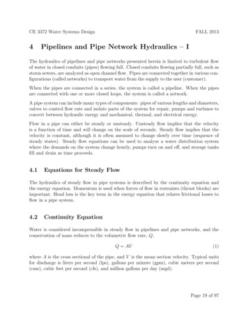
CE 3372 Water Systems DesignFALL 2013The roughness height is 0.00085 from the table on the Moody chart (in this document),so the roughness ratio is 0.00085 0.0017(13)D0.5Figure 16: Moody-Stanton Diagram annotated with Example 1 components.Figure 16 is the Moody chart with the roughness ratio shown as the light blue (cyan) curve,Page 30 of 97
CE 3372 Water Systems DesignFALL 2013the reynolds number as the black line, and the recovered friction factor (f 0.024) from themagenta line.To complete the analysis, we then use the Darcy-Weisbach equation for estimate the headloss asQ2(1cf s)2hl 8f L 2 5 8(0.024)(2000f t) 2 38.6f t(14)π gDπ (32.2f t/s2 )(0.5f t)5Now to compute the pressure drop, we simply account for the elevation change and whatremains must be pressure. First the change in elevation is about 2000sin5o 175f t. Thechange in pressure is therefore p ρg(hl (z2 z1 )) (38.6f t 175f t)(62.4)(0.9) 11, 999lb/f t2 83psi(15)Thus the oil pressure must be at least 83 psi greater at the lower elevation than the upperelevation for the oil to flow up the pipe. Find Q given hf , D, This type of problemrequires iteration if using the Moody chart, but it usually converges in two attempts. Thealternative is to use one of the explicit equations in a later section. The engineer computesthe Then computes the roughness ratio from the tabulated for the pipe material. Thenmakes a guess as to the flow rate, uses that guess to compute a Reynolds number, and lookup a friction factor and compute the head loss. If the computed value is too large, then theflow rate is reduced; if too small then increased. The trial-and-error process is greatly helpedby using a spreadsheet to record the various computations.Example An 80-foot horizontal, 1/2-inch diameter wrought iron pipe has an observed headloss of 40 feet. Estimate the discharge in the pipe.Solution Apply Darcy-Weisbach directly — the pipe is horizontal so the energy equation isquite boring,hl p 40f tρg(16)First compute the roughness height ratio — it will be needed to look up friction factors. 0.00015f t 0.0036D0.5i/12f t(17)Then construct a table of computations as shown in Table 2. Increase (decrease) the flowrate until the computed head loss is about the same as the required head loss. The moodychart is used the same way as in the previous example. The engineer will need to exercisesome judgement of when to stop, because as one gets close to the specified head loss, theability to read changes in f diminishes.Page 31 of 97
CE 3372 Water Systems DesignFALL 2013Table 1: Computation table for Estimating Q from head loss and material properties.QguessRedfhl guess30.0012.83 100.036 0.5740.0051.41 100.032 12.70.0082.26 1040.031 31.640.0092.25 100.030 37.9The result in this example is that the pipe discharge is about 0.009 cfs. Find D given Q, hf , The last kind of case is finding (design) the diameter required to move a specified volumeof water given a specified working head and pipe material. In this kind of problem, theengineer must guess a diameter, then compute Red based on the flow rate and the diameter.The engineer must also compute D . Then the engineer enters the Moody chart with thesetwo values (guesses), reads the friction factor and computed the head loss. If the headloss from the guess is too large, then the diameter is increased, too small then decreased.Upon convergence, the next larger commercially available diameter is selected for practicalapplication.Example An 600 foot wrought-iron pipe is to carry water at 20o C at a discharge of 3 CFS.The pipe drops 60 feet in the direction of flow and the desired pressure drop is 6 feet of head.What diameter pipe will function under these conditions?Solution Figure 17 is a sketch of the situation.Figure 17: Sketch for ExampleThe energy equation for this situation is(p1p2 ) (z1 z2 ) hlρg ρg(18)The elevation change is given as 60 feet and the pressure drop is given as 6 feet (that is thepressure is greater at location 1 by 6 feet than location 2). Thus the Darcy-Weisbach headPage 32 of 97
CE 3372 Water Systems DesignFALL 2013loss equation ishl 8f LQ2 66f tπ 2 gD5(19)As in the prior example, a computation table is useful. The sixth column is a computationaltrick to make a hand calculations faster. The term hfl is evaluated by taking the DarcyWeisbach equation and dividing out the friction factor (i.e.hlf2 8L π2QgD5 )Table 2: Computation table for Estimating D from head loss, discharge and material properties.hl fhlDguessRedDf0.250.500.511.41 1067.06 1056.92 1050.00060.00030.000290.0180.0160.0161.39 1054.35 1033.94 103 2500 69.6 63.0The result after three tries is that the diameter is between 6-7 inches, commercially available7 inch iron pipe exists8 , so this size could be specified in such a situation.5.2Head Loss Models – Hazen-WilliamsThe Hazen-Williams head loss model is another common model in civil engineering practice.It is an empirical model valid only for water, and is not for use with other liquids. Itappears in the Texas Administrative Code and has been used for water distribution systemsdesign for at least a century.Equation 20 is the formula that relates pipe velocity to head loss.V 1.381 Ch R0.63 S 0.54(20)where, V is the mean section velocity in feet per second, Ch is the Hazen-WIlliams losscoefficient (tabulated), R is the hydraulic radius in feet, and S hf /L is the slope of theenergy grade line (head loss per unit length)If Equation 20 is rearranged, a formal head loss equation results, as in Equation 21 forcircular pipes of diameter D in feet.hf 3.02 L D 1.167 (8V 1.85)Ch(21)7-inch pipe is uncommon, but is reported on NPS tables; so the pipe is commercially available somewhere.Page 33 of 97
CE 3372 Water Systems DesignFALL 2013More useful is the head loss in discharge form for circular pipes with discharge Q is cubicfeet per second.hf 3.02 L D 1.167 (4Q 1.85)πD2 Ch(22)The loss coefficients are tabulated in many places and are usually based on material type(cement, steel, etc.) and an estimate of age. Table 3 is one such tabulation9 , and is a ratherextensive list. The model is intended for pipes in sizes from 2-inches to 6-feet; outside theseranges the model may not be applicable.Table 3: Hazen-Williams Coefficients for Different Materials.MaterialABS - Acrylonite Butadiene StyreneAsbestos CementBrassCast-Iron - new unlined (CIP)Cast-Iron 20 years oldCast-Iron 40 years oldCast-Iron, cement linedCast-Iron, wrought plainCement liningConcrete lined, steel formsConcrete, oldCorrugated MetalDuctile Iron, cement linedFiber Glass Pipe - FRPGlassMetal Pipes - Very to extremely smoothPolyethylene, PE, PEHSmooth PipesSteel, corrugatedSteel, interior riveted, no projecting rivetsSteel, vitrified, spiral-rivetedTinWrought iron, plainWood StaveCh130140130 - 14013089 - 10064-83140100130 - 140140100 - 11060120150130130 - 1401401406011090 - 110130100110 - 120MaterialAluminumAsphalt LiningBrick sewerCast-Iron 10 years oldCast-Iron 30 years oldCast-Iron, asphalt coatedCast-Iron, bituminous linedCast-Iron, seal-coatedConcreteConcrete lined, wooden formsCopperDuctile Iron Pipe (DIP)FiberGalvanized ironLeadPlasticPolyvinyl chloride, PVC, CPVCSteel new unlinedSteel, welded and seamlessSteel, projecting girth and horizontal rivetsSteel, welded and seamlessVitrified ClayWooden or Masonry Pipe - SmoothCh130 - 150130 - 14090 - 100107 - 11375 - 90100140120100 - 140120130 - 140140140120130 - 140130 - 150150140 - 150100100100110120Example Estimate the head loss in a 72-inch, 10,000-foot steel pipe carrying water at 200CFS using the Hazen-Williams formula.Solution Using Table 3 an estimate of the Ch is 100. Next substitute into the HW formulaas4(200cf s) 1.85hf 3.02 (10, 000f t) (6f t) 1.167 () 28f t(23)π(6f t)2 1009Adapted from oefficients-d 798.html.Page 34 of 97
CE 3372 Water Systems Design5.35.3.1FALL 2013Head Loss Models – Manning’sNon-circular conduitsHydraulic radius concept.5.4Head Loss Models – Explicit EquationsAn alternative to the Moody chart are explicit equations based on regression models of thedata represented by the Moody chart. These equations are useful in programming solutionsto common pipe-flow design problems.5.4.1Friction Factor FormulasEquation 24 is the formula for friction factor for laminar flow (Red 2000).f 64Red(24)Equation 25 is the formula for friction factor for transitional to fully rough flow for the rangesof Red and roughness ratio shown (CITE SOURCE).f 0.25keD[log10 ( 3.7 (25)5.74 2)]Re0.9dvalid for : 4,000 Red 100,000,000 and 0.00001 5.4.2 D 0.002.Discharge FormulaCombining Equation 25 and Equation 9, then rearranging to isolate the discharge Q producesan explicit formula for estimating discharge from head loss and material properties. Equation26 is such an explicit formula (CITE SOURCE).q 1.78ν5/2pQ 2.22D ghf /L [log10 ( )](26)3/23.7D Dghf /LPage 35 of 97
CE 3372 Water Systems Design5.4.3FALL 2013Diameter FormulaA formula for diameter is also available. Equation 27 is a formula to estimate the requiredpipe diameter for a particular discharge, head loss, and roughness (CITE SOURCE).D 0.66[ 1.25 (LQ2 4.75L 5.2 0.04) νQ9.4 () ]ghfghf(27)Page 36 of 97
CE 3372 Water Systems Design5.5FALL 2013Head Losses in Bends and Fittings — (aka Minor Losses)In addition to head loss in the conduit, other losses are created by inlets, outlets, transitions,and other connections in the system. In fact such losses can be used to measure discharge(think of the orifice plate in the fluids laboratory). The fittings create additional turbulencethat generates heat and produces the head loss.Equation 28 is the typical loss modelhminor KV22g(28)where K is called a minor loss coefficient, and is tabulated (e.g. Table 4) for various kindsof fittings.Table 4: Minor Loss Coefficients for Different FittingsFitting TypeTee, Flanged, Line FlowTee, Threaded, Line FlowTee, Flanged, Branched FlowTee, Threaded , Branch FlowUnion, ThreadedElbow, Flanged Regular 90oElbow, Threaded Regular 90oElbow, Threaded Regular 45oElbow, Flanged Long Radius 90oElbow, Threaded Long Radius 90oElbow, Flanged Long Radius 45oReturn Bend, Flanged 180oReturn Bend, Threaded 180oGlobe Valve, Fully OpenAngle Valve, Fully OpenGate Valve, Fully OpenGate Valve, 1/4 ClosedGate Valve, 1/2 ClosedGate Valve, 3/4 ClosedSwing Check Valve, Forward FlowBall Valve, Fully OpenBall Valve, 1/3 ClosedBall Valve, 2/3 ClosedDiaphragm Valve, OpenDiaphragm Valve, Half OpenDiaphragm Valve, 1/4 OpenWater .150.262.11720.055.52002.34.3217The use is straightforward, and multiple fittings are summed in the loss term in the energyequation.Page 37 of 97
CE 3372 Water Systems DesignFALL 2013Example What is the pressure drop across a valve with nominal diameter of 8 cm, a losscoefficient of 3.2, and a flow rate of 0.04 m3 /sec?Solution First write the minor loss equation, solve for head loss.4 0.04 2( π(0.08)2)V2 (3.2) 10.3mhl K2g2(9.8)(29)Then convert the head loss into a pressure drop fromρg hl p 9800N/m3 10.3m 101, 321P a 101kP a5.6(30)Exercise Set1. A 5-foot diameter, enamel coated, steel pipe carries 60o F water at a discharge of 295cubic-feet per second (cfs). Using the Moody chart, estimate the head loss in a 10,000foot length of this pipe.2. Using the Moody chart, and the energy equation, estimate the diameter of a cast-ironpipe needed to carry 60o F water at a discharge of 10 cubic-feet per second (cfs) betweentwo reservoirs 2 miles apart. The elevation difference between the water surfaces inthe two reservoirs is 20 feet.3. Points A and B are 3 miles apart along a 24-inch ductile iron pipe carrying 50o F water.Point A is 30 feet higher in elevation than point B. The pressure at point B is 20pounds per square-inch (psi) greater than the pressure at point A. Using the Moodychart, and the energy equation, determine the direction and magnitude of flow (i.e.discharge and direction).4. (Writing Intensive Problem) Build and document10 a spreadsheet tool that implements the explicit formulas. Use the tool to repeat problems 1-3 and use these in yourdocumentation as tutorial examples for other users of your spreadsheet tool.10Use the spreadsheet report formatPage 38 of 97
CE 3372 Water Systems Design66.1FALL 2013Pipeline System Hydraulics – IIConduit SystemsConduit systems include pipes in series (which can already be analyzed methods presentedherein) as well as branching pipes, parallel pipes, manifolds, and networks.6.1.1Branching PipesFigure 18 is a sketch of a branched system. The three reservoirs are connected to a commonjunction (D) called a node. There are four unknowns, VAD , VBD , VDC , and pD /γ. TheFigure 18: Branched pipe systemtypical challenge is to find the flow (e.g. V A) in each of the three pipes and the pressure atthe junction. The fundamental relationships are energy loss in the branches, and continuityof flow at the node.Page 39 of 97
CE 3372 Water Systems DesignFALL 2013First energy along each pipe:zA zD 2pDLAD VAD fADγDAD 2g(31)zB zD 2pDLBD VBD fBDγDBD 2g(32)2pDLDC VDC zC fDCγDDC 2g(33)zD These three energy equations contain the four unknowns. For a unique solution to exist, weneed a fourth independent equation — in this instance, conservation of mass at the nodeprovides the fourth relation asAAD VAD ABD VBD ADC VDC(34)Now we have 4 equations in 4 unknowns; 3 equations happen to be nonlinear in an unknownand if one is solving by hand this is not a problem. If we use a computer spreadsheet, weneed to construct the quadratic term as V V , this ”vee times absolute vee” maintains thesign required to keep track of flow direction.ExampleConsider the branched system shown in Figure 19. In this example the friction factor isassumed constant for simplicity, but in practice would vary during the solution computations.Figure 19: Branched pipe systemThe hydraulics question is what is the discharge in each pipe and what is the total head atthe junction (notice we don’t know the junction elevation in this example — if the elevationwere specified, we could also find the pressure head).Page 40 of 97
CE 3372 Water Systems DesignFALL 2013Solution First populate the four equations with the appropriate numerical values.70 hD (0.015)5000 VAD VAD 0.6 2(9.8)(35)3000 VBD VBD 0.8 2(9.8)(36)100 hD (0.015) 80 hD (0.015)4000 VDC VDC 1.2 2(9.8)(37)π(0.6)2π(0.8)2π(1.2)2VAD VBD VDC444(38)Next, compute all the constants, and organize the 4 equations into a system of simultaneousequationshD 6.377VAD VAD 00 70hD02.869VBD VBD 0 100(39)hD00 2.551VDC VDC 8000.2827VAD0.5026VBD 1.1309VDC 0Because the system is non-linear we need to employ some tricks. First, it is a quadraticsystem so if a solution exists, Excel solver should be able to find one.First a more conventional vector-matrix structure 1 6.377 VAD 00hD70 1 1 02.869 VBD 0 VAD 100 2 100 2.551 VDC VBD 80 3 00.28270.5026 1.1309VDC0 4(40)Now we can use solver to find a solution. We notice that the right-hand-side is a vector of“errors”. If we square these values and sum them ( T ), then minimize this sum of squarederrors by changing hD , VAD , VBD , and VDC , the result should be the solution (if the error issmall enough).Figure 20 is a screen capture of an Excel worksheet before starting the solution algorithm.Notice the column labeled X contains an initial guess for the unknowns.Page 41 of 97
CE 3372 Water Systems DesignFALL 2013Figure 20: Branched pipe system — Excel solution set-upPage 42 of 97
CE 3372 Water Systems DesignFALL 2013After building the spreadsheet and preparing the columns, then the engineer must selectsolver to minimize the error vector (the last column in the worksheet). The SOLVER addin does the job nicely, GOAL SEEK might work, but provides less control of precision andstopping criterion.Figure 21: Branched pipe system — Excel solution select solverFigure 21 is the solver set-up for this example. When the engineer selects SOLVE thenthe program will attempt to minimize the error by changing values of the X vector. Theexample does NOT use program defaults, but instead reduces the tolerance and precisionvalues (in the Options section) and chooses the conjugate-gradient direction finding methodand centered differences.Finally, when the solver is completed, we recover the solution by multiplying the resultsby pipe areas to obtain the flows. Figure 22 is the solution for this example (the arithmetic was added at the bottom after the program converged to the near-zero ”sum-squarederror”).Page 43 of 97
CE 3372 Water Systems DesignFALL 2013Figure 22: Branched pipe system — Excel solutionThe results are:1. QAD 0.381m3 /s, from Node D to Reservior A (opposite the original assumeddirection).2. QBD 1.273m3 /s, from Reservoir B to the node (the assumed flow direction in thispipe).3. QDC 0.89m3 /s from the Node D to reservoir C (the assumed direction in this pipe).4. hD 81.6m.An alternate solution approach is to guess values of hD and use the energy equations tofind re
ow equations can be used to analyze a water distribution system where the demands on the system change hourly, pumps turn on and o , and storage tanks ll and drain as time proceeds. 4.1 Equations for Steady Flow The hydraulics of steady ow in pipe systems is described by the continuity eq