Transcription
An overview of the Hydraulicsof Water Distribution NetworksJune 21, 2017by Bassam Kassab, P.E.Senior Water Resources Specialist, Santa Clara Valley Water DistrictAdjunct Faculty, San José State University1
Outline Pressurized vs. open-channel flow in closed conduitsUniform vs. nonuniform flow & steady vs. unsteady flowConservation of mass principleConservation of energy principle: Friction and minor headlossesWhat about HGL and EGL?Water distribution network analysisSoftware for steady-state analysis and extended-period simulationsPumps and turbinesHydraulic transients (surge analysis)Hydraulic transients softwareReferencesContact informationQ&A sessionBassam Kassab2
Pressurized vs. open-channel flowin closed conduitsPressurized flowOpen-channel flowDriven by head differential and/orpump(s)Gravity drivenReynolds number (Re): Laminar,transition zone or wholly turbulentFroude Number (Fr): Subcritical,critical or supercritical flowFriction loss: Darcy-Weisbach’s,Friction loss: Manning’sHazen-Williams’ or Chezy’s equation equationBassam Kassab3
Reynolds Number Reynolds Number (ratio of inertia force to viscous force) V velocity (m/s or ft/sec)D pipe diameter (m or ft) density of fluid (Kg/m3 or lbm/ft3) dynamic viscosity of fluid (N.s/m2 or lbf.s/ft2) kinematic viscosity (m2/s or ft2/s)Re Bassam KassabVD VD 4
Laminar vs. turbulent flow Re 2,000: laminar flow Re from 4,000 to 800,000,000 (or more): turbulent flow(transition zone and wholly turbulent zone)Bassam Kassab5
Moody Diagram6
Uniform vs. Nonuniform Flow& Steady vs. Unsteady Flow Uniform flow: Constant flow characteristics (like velocity) withrespect to space Nonuniform flow, like in the caseof changing pipe size Steady flow: Constant flow characteristics with respect to time.Steady flow is considered when designing a pipe network (lookingfor pressures at certain locations and velocities in the pipes) Consider unsteady (transient) phenomena to refine the design(pipe pressure class and thickness)Bassam Kassab7
Conservation of Mass Principle In a control volume:dS In Outdt(change in storage over time inflow – outflow) For steady & incompressible flow: dS/dt 0,continuity equation becomes:In Out (inflow outflow)i.e.,Bassam Kassab Qin Qout8
Conservation of Mass Principle Continuity equation applied to a pipe junction:Q1 Q2 Q3 Q4Bassam Kassab9
Conservation of Energy Principle In pipeline design, most often consider steady-state flow(does not vary with time). Energy equation is written as:p V 1212g z1 h pumpp V 2222g z 2 hturbine hlosses Steady-state Bernoulli’s Equation (no head loss nor gain)along a streamline:p VBassam Kassabg1212g z1 p Vg2222g z210
Conservation of Energy Principle Pressure head:p/ Elevation head:z Velocity head:V2/2g Piezometric head:p/ z(where is the specific weight of water: ρ g )(a.k.a. Hydraulic Grade Line or HGL) Total head:p/ z V2/2g(a.k.a. Energy Grade Line or EGL) Headlosses:hlosses friction headloss (hLf ) minor headloss (hLm) Turbine head:hturbine pressure head dissipated in a turbineto produce electric energy Pump head:hpump pressure head gained from a pumpBassam Kassab11
Friction Headloss Friction loss results from friction between the fluid and pipe wall The most useful headloss equation for pressurized pipe flow is theDarcy-Weisbach equation:PipelengthFrictionheadloss2hLfLV fD 2gDimensionlessfrictioncoefficientBassam ation12
Minor Headloss Minor headloss can be caused by the presence of a valve inthe network, entrance to a pipe from a reservoir, exit to atank, bend in the pipe, elbow, pipe expansion, pipecontraction (reducer), or other fittings Use a minor headloss coefficient (K) in the following minorheadloss expression:2Vh K 2gLmBassam Kassab13
Minor Loss14
ValvesA large butterfly valveshown as partially openHeadloss coefficient (K) for abutterfly valve(Bosserman and Hunt, 1998)2V KhLm 2 gBassam KassabWhen K is very large, minor headloss couldbecome larger than the major (friction) headloss.So the word “minor” is a misnomer15
What about HGL and EGL?The Supervisory Control And Data Acquisition (SCADA) systemrecords and reports on a screen various parameters data for apipe network, a treatment plant, etc. Parameters such as: flow,pressure and hydraulic grade line (HGL)Bassam Kassab16
What about HGL and EGL? EGL p/ z V2/2g HGL p/ z Test your knowledge: What does the distance between the twoarrows at “Profile X” represent? What does “h” refer to?Does the “Box” represent a pump or a turbine?Is the flow (discharge) in the pipeline going from left to right orvice versa? Explain your answer.Bassam Kassab17
Water Distribution Network AnalysisSource:Reference # 1 For the simple network shown above with 5 unknownflow values in the 5 pipes, we need to solve 5equations. These are: 3 linear continuity equations at 3 junctions, and 2 nonlinear energy equations along 2 paths. Solution of a nonlinear system of 5 equations is notstraightforwardBassam Kassab18
Water Distribution Network Analysis Hardy-Cross Method, 1936 (manual technique only suitable for small networks) Numerical Methods (like Newton-Raphson technique) use iterations but areprone to problems of diverging solutions Linearization Method (approximation) Perturbation Method (Basha & Kassab, 1996), a direct, mathematical solution:Bassam KassabSource:Reference # 119
Software for steady-state analysis& extended-period simulations (EPS) Hydraulic modeling software use numerical algorithms to obtainthe steady-state solution for a water distribution network EPS: used for water quality analysis (water age, contaminanttracing). EPS is simply a series of steady-solutions over time Free software: EPANET Commercial software (H2ONET, InfoMAP, WaterCAD,WaterGEMS, etc.) give same results as EPANET but haveadditional bells and whistles. Some have better graphic userinterface (GUI), others work in a GIS environment or can have anadd-on surge software.Bassam Kassab20
Skeletonizing a Water Distribution NetworkBassam KassabThe raw water distribution system of Santa Clara Valley WaterDistrict was modeled using H2ONET21
Pumps and Turbines Pumps and valves are easily modeled using commercialsoftware But it is important to have a solid understanding of pumpcurves, operating point concept, and pump efficiencyBassam Kassab22
Pumps Pump characteristic curve (pump head hp vs. flow Q): originally provided bymanufacturer, then updated by technicians/engineers who calibrate the pump regularly System curve: hp vs. Q as obtained from energy equation. Note that system curvechanges every time conditions change (like tank level fluctuates) Operating point: where the 2 curves meet Operating point is not always point of best (maximum) efficiencyBassam KassabSource:Reference # 223
Finding the Pump Operating PointSystem curve (a parabolic equation) for the case of a pump on a pipeconnecting two reservoirs/tanks:hBassam Kassabpump ( z z1 ) hLf hLm224
Pumps in Series & Pumps in Parallel For pumps in series: Pump head (hp) adds up but the flow Q remainsconstant For pumps in parallel: Flow (Q) adds up but pump head hp remains thesameBassam Kassab25
Pump Power and Efficiency Hydraulic power of a pump Q hp Etotal overall (total) pump efficiency output power /input power Hydraulic power / electric power Etotal Eo . Emotor . EpumpBassam Kassab26
Turbines Hydraulic power of a turbine Q hT ET Overall turbine efficiency ouput power / inputpower electric power / hydraulic powerBassam Kassab27
Hydraulic Transients (Surge Analysis) Hydraulic transients (aka waterhammers) are caused by asudden opening or closure of a valve, starting or stopping apump or a turbine, or accidental events, like power outage.Source:Reference # 3Bassam Kassab28
Hydraulic Transients (Surge Analysis)Solution by: Arithmetic Method (Joukowski, 1904), approximation Method of Characteristics (MOC), most popular Wave-Plan Analysis Method (Wood et al., 1966) Linear methods (approximation) Perturbation Method (Basha & Kassab, 1996), direct, mathematicalsolution (Reference 3)Diagram representing thesolution of a waterhammerproblem by the MOCBassam Kassab29
Hydraulic Transients (Surge Analysis)The solution by the Perturbation Method (a direct, mathematicalapproach) matches very well with the numerical MOCPressure head at the valve,as obtained by thePerturbation Method, for thecases of instantaneous,linear and exponential valveclosure scenarios and theircomparison to the numericalsolution by the MOCBassam KassabSource:Reference # 330
Hydraulic Transients (Surge Analysis)Another valve closure case:Solution by Wave CharacteristicMethod matches with MOCSource:Reference # 4Bassam Kassab31
Hydraulic Transients (Surge Analysis) To prevent transients: Slowly open and close of valves Properly close of fire hydrants Use pump controls to ramp pump speed up and down Lower pipeline velocities To control maximum and/or minimum pressures: Use surgetanks; air chambers; one-way tanks; pump bypass valves; reliefvalves; air inlet valvesSource:Reference # 4Bassam Kassab32
Hydraulic Transients Software Many software programs on the market. They rely on numericalmethods to solve the waterhammer equations Innovyze (previosuly MWH Soft) has: H2OSurge program (an add-on to H2ONET), and InfoSurge (add-on to InfoWater, in GIS environment)Bassam Kassab33
References1. H. A. Basha and B. G. Kassab, Analysis of water distributionsystems using a perturbation method. AppliedMathematical Modelling, 1996, 20 (4), 290-297.2. “Advanced Water Distribution Modeling and Management.”Haestad Methods, Waterbury, Connecticut, 2002.3. H. A. Basha and B. G. Kassab, A perturbation solution to thetransient pipe flow problem. Journal of Hydraulic Research,1996, 34 (5), 633-649.4. “Pressure Wave Analysis of Transient Flow in PipeDistribution Systems.” D. Wood, S. Lingireddy and P. Boulos,MWH Soft, Pasadena, California, 2005.Bassam Kassab34
Contact Information Bassam Kassab Email: bkassab@valleywater.org Webpage: www.sjsu.edu/people/bassam.kassabQ&A sessionBassam Kassab35
Jun 21, 2017 · An overview of the Hydraulics of Water Distribution Networks by Bassam Kassab, P.E. . (SCADA) system records and reports on a screen various parameters data for a pi