WIXLIB

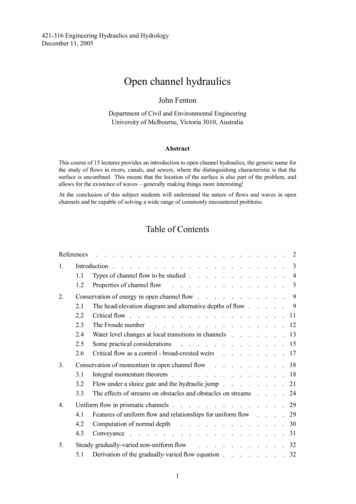
Open channel hydraulicsJohn Fentonbetween them as appropriate. In these sorts of problems we will assume that the slope of the streambalances the friction losses and we treat such problems as frictionless flow over a generally-horizontalbed, so that for the individual states between rapidly-varied regions we usually consider the flow to beuniform and frictionless, so that the whole problem is modelled as a sequence of quasi-uniform flowstates.Case (d) – Unsteady flow:Here conditions vary with time and position as a wave traverses thewaterway. We will obtain some results for this problem too.1.2 Properties of channel flowz ηzz z m inyFigure 1-2. Cross-section of flow, showing isovels, contours on which velocity normal to the section is constant.Consider a section of a waterway of arbitrary section, as shown in Figure 1-2. The x co-ordinate ishorizontal along the direction of the waterway (normal to the page), y is transverse, and z is vertical. Atthe section shown the free surface is z η , which we have shown to be horizontal across the section,which is a good approximation in many flows.1.2.1 Discharge across a cross-sectionThe volume flux or discharge Q at any point isQ Zu dA UAAwhere u is the velocity component in the x or downstream direction, and A is the cross-sectional area.This equation defines the mean horizontal velocity over the section U . In most hydraulic applicationsthe discharge is a more important quantity than the velocity, as it is the volume of water and its rate ofpropagation, the discharge, which are important.1.2.2 A generalisation – net discharge across a control surfaceHaving obtained the expression for volume flux across a plane surface where the velocity vector isnormal to the surface, we introduce a generalisation to a control volume of arbitrary shape bounded by acontrol surface CS. If u is the velocity vector at any point throughout the control volume and n̂ is a unitvector with direction normal to and directed outwards from a point on the control surface, then u · n̂ onthe control surface is the component of velocity normal to the control surface. If dS is an elemental areaof the control surface, then the rate at which fluid volume is leaving across the control surface over that5

Open channel hydraulicsJohn Fentonelemental area is u · n̂ dS , and integrating givesTotal rate at which fluid volume is leaving across the control surface ZCS(1.1)u · n̂ dS.If we consider a finite length of channel as shown in Figure 1-3, with the control surface made up ofn̂1u2u1n̂ 2Figure 1-3. Section of waterway and control surface with vertical endsthe bed of the channel, two vertical planes across the channel at stations 1 and 2, and an imaginaryenclosing surface somewhere above the water level, then if the channel bed is impermeable, u · n̂ 0there; u 0 on the upper surface; on the left (upstream) vertical plane u · n̂ u1 , where u1 isthe horizontal component of velocity (which varies across the section); and on the right (downstream)vertical plane u · n̂ u2 . Substituting into equation (1.1) we haveZZTotal rate at which fluid volume is leaving across the control surface u1 dA u2 dAA1A2 Q1 Q2 .If the flow is steady and there is no increase of volume inside the control surface, then the total rate ofvolume leaving is zero and we have Q1 Q2 .While that result is obvious, the results for more general situations are not so obvious, and we willgeneralise this approach to rather more complicated situations – notably where the water surface in theControl Surface is changing.1.2.3 A further generalisation – transport of other quantities across the control surfaceWe saw that u · n̂ dS is the volume flux through an elemental area – if we multiply by fluid density ρ thenρ u · n̂ dS is the rate at which fluid mass is leaving across an elemental area of the control surface, witha corresponding integral over the whole surface. Mass flux is actually more fundamental than volumeflux, for volume is not necessarily conserved in situations such as compressible flow where the densityvaries. However in most hydraulic engineering applications we can consider volume to be conserved.Similarly we can compute the rate at which almost any physical quantity, vector or scalar, is beingtransported across the control surface. For example, multiplying the mass rate of transfer by the fluidvelocity u gives the rate at which fluid momentum is leaving across the control surface, ρu u · n̂ dS .1.2.4 The energy equation in integral form for steady flowBernoulli’s theorem states that:In steady, frictionless, incompressible flow, the energy per unit mass p/ρ gz V 2 /2 is constant6

Open channel hydraulicsJohn Fentonalong a streamline,where V is the fluid speed, V 2 u2 v2 w2 , in which (u, v, w) are velocity components in a cartesianco-ordinate system (x, y, z) with z vertically upwards, g is gravitational acceleration, p is pressure andρ is fluid density. In hydraulic engineering it is usually more convenient to divide by g such that we saythat the head p/ρg z V 2 /2g is constant along a streamline.In open channel flows (and pipes too, actually, but this seems never to be done) we have to considerthe situation where the energy per unit mass varies across the section (the velocity near pipe walls andchannel boundaries is smaller than in the middle while pressures and elevations are the same). In thiscase we cannot apply Bernoulli’s theorem across streamlines. Instead, we use an integral form of theenergy equation, although almost universally textbooks then neglect variation across the flow and referto the governing theorem as ”Bernoulli”. Here we try not to do that.The energy equation in integral form can be written for a control volume CV bounded by a controlsurface CS, where there is no heat added or work done on the fluid in the control volume:ZZ ρ e dV (p ρe) u.n̂ dS 0,(1.2) tCVCS{z}{z} Rate at which energy is increasing inside the CVRate at which energy is leaving the CSwhere t is time, ρ is density, dV is an element of volume, e is the internal energy per unit mass of fluid,which in hydraulics is the sum of potential and kinetic energiese gz 1¡ 2u v 2 w2 ,2where the velocity vector u (u, v, w) in a cartesian coordinate system (x, y, z) with x horizontallyalong the channel and z upwards, n̂ is a unit vector as above, p is pressure, and dS is an elemental areaof the control surface.Here we consider steady flow so that the first term in equation (1.2) is zero. The equation becomes:Z ³ ρ¡ 2p ρgz u v 2 w2 u.n̂ dS 0.2CSWe intend to consider problems such as flows in open channels where there is usually no importantcontribution from lateral flows so that we only need to consider flow entering across one transverse faceof the control surface across a pipe or channel and leaving by another. To do this we have the problemof integrating the contribution over a cross-section denoted by A which we also use as the symbol forthe cross-sectional area. When we evaluate the integral over such a section we will take u to be thevelocity along the channel, perpendicular to the section, and v and w to be perpendicular to that. Thecontribution over a section of area A is then E , where E is the integral over the cross-section:Z ³ ρ¡ 2p ρgz u v2 w2 u dA,E (1.3)2Aand we take the depending on whether the flow is leaving/entering the control surface, because u.n̂ u. In the case of no losses, E is constant along the channel. The quantity ρQE is the total rate ofenergy transmission across the section.Now we consider the individual contributions: R ¡(a) Velocity head term ρ2 A u2 v2 w2 u dAIf the flow is swirling, then the v and w components will contribute, and if the flow is turbulent therewill be extra contributions as well. It seems that the sensible thing to do is to recognise that all velocitycomponents and velocity fluctuations will be of a scale given by the mean flow velocity in the stream at7

Open channel hydraulicsJohn Fentonthat point,and so we simply write, for the moment ignoring the coefficient ρ/2:Z¡ 2 Q3u v 2 w2 u dA αU 3 A α 2 ,A(1.4)Awhich defines α as a coefficient which will be somewhat greater than unity, given by R ¡ 222 u dAA u v w.α U 3A(1.5)Conventional presentations define it as being merely due to the non-uniformity of velocity distributionacross the channel:Ru3 dA,α A 3U Ahowever we suggest that is more properly written containing the other velocity components (and turbulent contributions as well, ideally). This coefficient is known as a Coriolis coefficient, in honour of theFrench engineer who introduced it.Most presentations of open channel theory adopt the approximation that there is no variation of velocityover the section, such that it is assumed that α 1, however that is not accurate. Montes (1998, p27)quotes laboratory measurements over a smooth concrete bed giving values of α of 1.035-1.064, whilefor rougher boundaries such as earth channels larger values are found, such as 1.25 for irrigation canalsin southern Chile and 1.35 in the Rhine River. For compound channels very much larger values may beencountered. It would seem desirable to include this parameter in our work, which we will do.(b) Pressure and potential head termsThese are combined asZ(p ρgz) u dA.(1.6)AThe approximation we now make, common throughout almost all open-channel hydraulics, is the ”hydrostatic approximation”, that pressure at a point of elevation z is given byp ρg height of water above ρg (η z) ,(1.7)where the free surface directly above has elevation η . This is the expression obtained in hydrostatics fora fluid which is not moving. It is an excellent approximation in open channel hydraulics except wherethe flow is strongly curved, such as where there are short waves on the flow, or near a structure whichdisturbs the flow. Substituting equation (1.7) into equation (1.6) givesZρg η u dA,Afor the combination of the pressure and potential head terms. If we make the reasonable assumption thatη is constant across the channel the contribution becomesZρgηu dA ρgηQ,Afrom the definition of discharge Q.(c) Combined termsSubstituting both that expression and equation (1.4) into (1.3) we obtainµ¶α Q2E ρgQ η ,2g A28(1.8)

Open channel hydraulicsJohn Fentonwhich, in the absence of losses, would be constant along a channel. This energy flux across entry andexit faces is that which should be calculated, such that it is weighted with respect to the mass flow rate.Most presentations pretend that one can just apply Bernoulli’s theorem, which is really only valid alonga streamline. However our results in the end are not much different. We can introduce the concept of theMean Total Head H such thatH Energy fluxα Q2E η ,g Mass fluxg ρQ2g A2(1.9)which has units of length and is easily related to elevation in many hydraulic engineering applications,relative to an arbitrary datum. The integral version, equation (1.8), is more fundamental, although incommon applications it is simpler to use the mean total head H , which will simply be referred to as thehead of the flow. Although almost all presentations of open channel hydraulics assume α 1, we willretain the general value, as a better model of the fundamentals of the problem, which is more accurate,but also is a reminder that although we are trying to model reality better, its value is uncertain to a degree,and so are any results we obtain. In this way, it is hoped, we will maintain a sceptical attitude to theapplication of theory and ensuing results.(d) Application to a single length of channel – including energy lossesWe will represent energy losses by E . For a length of channel where there are no other entry or exitpoints for fluid, we havegiving, from equation (1.8):Eout Ein E,µ¶µ¶α Q2α Q2ρQout gη ρQin gη E,2 A2 out2 A2 inand as there is no mass entering or leaving, Qout Qin Q, we can divide through by ρQ and by g , asis common in hydraulics:µ¶¶µα Q2α Q2η η H,2g A2 out2g A2 inwhere we have written E ρgQ H , where H is the head loss. In spite of our attempts to useenergy flux, as Q is constant and could be eliminated, in this head form the terms appear as they are usedin conventional applications appealing to Bernoulli’s theorem, but with the addition of the α coefficients.2. Conservation of energy in open channel flowIn this section and the following one we examine the state of flow in a channel section by calculating theenergy and momentum flux at that section, while ignoring the fact that the flow at that section might beslowly changing. We are essentially assuming that the flow is locally uniform – i.e. it is constant alongthe channel, / x 0. This enables us to solve some problems, at least to a first, approximate, order.We can make useful deductions about the behaviour of flows in different sections, and the effects ofgates, hydraulic jumps, etc. Often this sort of analysis is applied to parts of a rather more complicatedflow, such as that shown in Figure 1-1(c) above, where a gate converts a deep slow flow to a faster shallowflow but with the same energy flux, and then via an hydraulic jump the flow can increase dramatically indepth, losing energy through turbulence but with the same momentum flux.2.1 The head/elevation diagram and alternative depths of flowConsider a steady ( / t 0) flow where any disturbances are long, such that the pressure is hydrostatic. We make a departure from other presentations. Conventionally (beginning with Bakhmeteff in1912) they introduce a co-ordinate origin at the bed of the stream and introduce the concept of ”specificenergy”, which is actually the head relative to that special co-ordinate origin. We believe that the use of9

Open channel hydraulicsJohn Fentonthat datum somehow suggests that the treatment and the results obtained are special in some way. Also,for irregular cross-sections such as in rivers, the ”bed” or lowest point of the section is poorly defined,and we want to minimise our reliance on such a point. Instead, we will use an arbitrary datum for thehead, as it is in keeping with other areas of hydraulics and open channel theory.Over an arbitrary section such as in Figure 1-2, from equation (1.9), the head relative to the datum canbe writtenαQ2 1,H η (2.1)2g A2 (η)where we have emphasised that the cross-sectional area for a given section is a known function of surfaceelevation, such that we write A(η). A typical graph showing the dependence of H upon η is shown inFigure 2-1, which has been drawn for a particular cross-section and a constant value of discharge Q,such that the coefficient αQ2 /2g in equation (2.1) is constant.H ηη11SurfaceelevationηηcH η η22αQ212g A2 (η)zminHcHead H E/ρgQFigure 2-1. Variation of head with surface elevation for a particular cross-section and dischargeThe figure has a number of important features, due to the combination of the linear increasing functionη and the function 1/A2 (η) which decreases with η . In the shallow flow limit as η zmin (i.e. the depth of flow, and hence the cross-sectional areaA(η), both go to zero while holding discharge constant) the value of H αQ2 /2gA2 (η) becomesvery large, and goes to in the limit. In the other limit of deep water, as η becomes large, H η , as the velocity contribution becomesnegligible. In between these two limits there is a minimum value of head, at which the flow is called criticalflow, where the surface elevation is η c and the head Hc . For all other H greater than Hc there are two values of depth possible, i.e. there are two differentflow states possible for the same head. The state with the larger depth is called tranquil, slow, or sub-critical flow, where the potential tomake waves is relatively small. The other state, with smaller depth, of course has faster flow velocity, and is called shooting, fast, orsuper-critical flow. There is more wave-making potential here, but it is still theoretically possiblefor the flow to be uniform. The two alternative depths for the same discharge and energy have been called alternate depths.10

Open channel hydraulicsJohn FentonThat terminology seems to be not quite right – alternate means ”occur or cause to occur by turns,go repeatedly from one to another”. Alternative seems better - ”available as another choice”, andwe will use that. In the vicinity of the critical point, where it is easier for flow to pass from one state to another, theflow can very easily form waves (and our hydrostatic approximation would break down). Flows can pass from one state to the other. Consider the flow past a sluice gate in a channel asshown in Figure 1-1(c). The relatively deep slow flow passes under the gate, suffering a largereduction in momentum due to the force exerted by the gate and emerging as a shallower fasterflow, but with the same energy. These are, for example, the conditions at the points labelled 1 and2 respectively in Figure 2-1. If we have a flow with head corresponding to that at the point 1 withsurface elevation η1 then the alternative depth is η 2 as shown. It seems that it is not possible togo in the other direction, from super-critical flow to sub-critical flow without some loss of energy,but nevertheless sometimes it is necessary to calculate the corresponding sub-critical depth. Themathematical process of solving either problem, equivalent to reading off the depths on the graph,is one of solving the equationαQ2αQ2 η η2 12gA2 (η 1 )2gA2 (η 2 ) {z} {z}H1(2.2)H2for η2 if η 1 is given, or vice versa. Even for a rectangular section this equation is a nonlinear transcendental equation which has to be solved numerically by procedures such as Newton’s method.2.2 Critical flowBδηδAFigure 2-2. Cross-section of waterway with increment of water levelWe now need to find what the condition for critical flow is, where the head is a minimum. Equation (2.1)isα Q2,H η 2g A2 (η)and critical flow is when dH/dη 0:dHαQ2dA 1 0.3dηgA (η)dηThe problem now is to evaluate the derivative dA/dη . From Figure 2-2, in the limit as δη 0 theelement of area δA B δη,such that dA/dη B , the width of the free surface. Substituting, we havethe condition for critical flow:αQ2 B 1.gA311(2.3)

Open channel hydraulicsJohn FentonThis can be rewritten asα(Q/A)2 1,g (A/B)and as Q/A U , the mean velocity over the section, and A/B D, the mean depth of flow, this meansthatCritical flow occurs when αU2 1,gDthat is, when α We write this asαF 2 1 or(Mean velocity)2 1.g Mean depth αF 1,(2.4)(2.5)where the symbol F is the Froude number, defined by:Mean velocityUQ/A F p. g Mean depthgDgA/BThe usual statement in textbooks is that ”critical flow occurs when the Froude number is 1”. We havechosen to generalise this slightly by allowing for the coefficient α not necessarily being equal to 1, givingαF 2 1 at critical flow. Any form of the condition, equation (2.3), (2.4) or (2.5) can be used. The meandepth at which flow is critical is the ”critical depth”:Dc αQ2U2 α 2.ggA(2.6)2.3 The Froude numberThe dimensionless Froude number is traditionally used in hydraulic engineering to express the relativeimportance of inertia and gravity forces, and occurs throughout open channel hydraulics. It is relevantwhere the water has a free surface. It almost always appears in the form o

Open channel hydraulics John Fenton recognise that we can treat this approximately, but it remains an often-unknown aspect of each problem. This reminds us that we are obtaining approximate solutions