WIXLIB

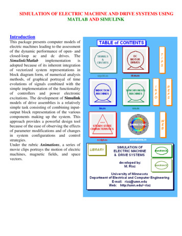
SIMULATION OF ELECTRIC MACHINE AND DRIVE SYSTEMS USINGMATLAB AND SIMULINKIntroductionThis package presents computer models ofelectric machines leading to the assessmentof the dynamic performance of open- andclosed-loop ac and dc drives. TheSimulink/Matlabimplementationisadopted because of its inherent integrationof vectorized system representations inblock diagram form, of numerical analysismethods, of graphical portrayal of timeevolutions of signals combined with thesimple implementation of the functionalityof controllers and power electronicexcitations. The development of Simulinkmodels of drive assemblies is a relativelysimple task consisting of combining inputoutput block representation of the variouscomponents making up the system. Thisapproach provides a powerful design toolbecause of the ease of observing the effectsof parameter modifications and of changesin system configurations and controlstrategies.Under the rubric Animations, a series ofmovie clips portrays the motion of electricmachines, magnetic fields, and spacevectors.

The approachElectric machinesThe starting step in the mathematical modeling of ac machines is to describe them ascoupled stator and rotor polyphase circuits in terms of so-called phase variables,namely stator currents ias, ibs, ics; rotor currents iar, ibr, icr for an induction machine or if,ikd, ikq for a synchronous machine; the rotor speed ωm ; and the angular displacement θbetween stator and rotor windings. The magnetic coupling is expressed in terms of aninductance matrix which is a function of position θ. The matrix expression of themachine equations are readily formulated in Matlab or Simulink language. A detailedexample of this approach is given in a later section.The next step is to transform the original stator and rotor abc frames of reference into acommon k or dq frame in which the new variables for voltages, currents, and fluxescan be viewed as 2-D space vectors. In this common frame the inductances becomeconstant independent of position. Figure 1 illustrates various reference frames(coordinate systems): the triplet [As Bs Cs] denotes a three-phase system attached tothe stator while the pair [as bs] corresponds to an equivalent two-phase system (zerosequence components can be ignored in Y-connected ac machines in which the neutralis normally isolated). Among possible choices of dq frames are the following:a) Stator frame where ωk 0b) Rotor frame where ωk ωmc) Synchronous frame associated with the frequency ωs (possibly time varying)of the stator excitation.d) Rotor flux frame in which the d-axis lines up with the direction of the rotorflux vector.The choice of the common dq frame is usually dictated by the symmetry constraintsimposed by the construction and excitation of the machine. With the completesymmetry encountered in a three-phase induction machine with balanced sinusoidalexcitation, any one of the five frames can be used, although the synchronous frame ismore convenient in as much as all signals appear as constant dc in steady state.However, certain control strategies may require the adoption of a specific frame, as isthe case of vector control where the reference frame is attached to the rotor flux vector.In the presence of asymmetry, the common frame is attached to the asymmetricalmember: an induction motor with unbalanced excitation or asymmetrical statorwindings (the case of a capacitor motor) will be modeled in the stator frame where as asynchronous machine is represented in the rotor frame. In the common dq frame, themachine dynamic equations appear as differential equations with constant coefficients(independent of rotor position) and nonlinearities confined to products of variablesassociated with speed voltages and torque components.

Figure 1. Reference frames in ac machine analysisω denotes the rotational speed or angular frequency of a frame (in electrical rad/s)with respect to the stationary stator. The angular position is obtained by integratingspeed over time, that is θ ω dt .

Excitations and controllersThe simulation of the inputs to the machines involves the mathematical representationof programmed time sequence of events such as the sudden application or removal ofmechanical loads, the ramping of the magnitude and frequency of the applied voltages, oreven the changes in parameter values (for instance, rotor resistance). Similarly thefunctionality of power electronics type of excitations can generally be realized in the form ofsimple mathematical expressions: as an example, a PWM signal can be described by thefunctionsignum[m - tri(t)] where m is the modulation factor ( 1 m 1) and2tri(t) sin 1[sin(ωt γ )] is a triangular waveform of unit amplitude,πfrequency ω, and phase γThis function is readily translated into Simulink block form.The simulation of speed or position controllers in drive systems is achieved by using a relayblock in a hysteresis type of controller, and a simple combination of gains, summers andintegrator (incorporating limiters to include antiwindup features) in a PI type of controller.Initial conditionsInitial conditions are established by specifying a steady-state operating condition. Thesimplest case is encountered in the simulation of the starting of a motor for which all initialconditions are zero. In some other case, the initial conditions can simply be calculated beforerunning the simulation: for example, under steady-state sinusoidal excitation, an inductionmotor running at a specified speed can be quickly analyzed in terms of a standard phasorequivalent circuit; by using phasor techniques, one can compute the corresponding loadtorque and initial conditions. However, in most instances, a specified operating condition canonly be obtained after running the simulation for a time that will depend on the startingsetting of these initial conditions. This situation will occur if, in the above case of theinduction motor, torque instead of speed is specified or if the mechanical load is a nonlinearfunction of speed. This is the normal situation encountered with power electronic inputsignals: a steady-state condition is reached when an output signal waveform is repeated everyswitching cycle so that the values at the beginning and end of a cycle are equal. When asteady-state condition is attained, one can then save this so-called final state and use it later asthe initial state in a renewed simulation which now includes the specified time sequencedinput events.

Space vector model of the induction machine(SI units)Electrical system equations:dλ sv s Rs i s ωkMλ sdtdλrv r Rr i r (ωk ωm )Mλrdt fd 0πwhere the space vector f and the rotational operator M 2 1 fq 1 0 Flux linkage-current relations:or i s Γ s λ s Γm λrλ s L s i s Lm i rλ r Lm i s Lr i ri r Γm λ s Γr λrLLLand Γ s r Γr swhere L s Lm L slΓm m Lr Lm Lrl LmLsl LmLrl LslLrlMechanical system equations:dωTe J mec Bmωmec TLdtwhere Te k(λ s i s ) k(Mλ s i s ) (λ dsiqs λ qsids ) k( i r λr ) kLm ( i r i s ) kandωmec 2ωmpk Lm( λ r i s ) kΓm ( λ r λ s )Lr3p22Nomenclature:v voltage space vector [V]i current space vector [A]λ flux linkage space vector [Wb]R Resistance [Ω]L Inductance [H]-1Γ Inverse inductance [H ]f0 Base frequency [Hz]operators: cross productr rotorsubscripts: s statorωo 2πfo Base frequency [rad/s]ωk speed of dq frame [rad/s]]ωm rotor speed [rad/s]Te electromagnetic torque [N.m]TL load torque [N.m]J moment of inertia [kg.m2]p number of polesM rotation dot productd direct axis q quadrature axis

Simulink block diagram modelThese mathematical equations can be represented as shown below in a block diagramform that preserves the one-to-one correspondence between the 2D space vectors ofthe equations and the vectorized signals (of width 2) appearing in the Simulinkrepresentation. It is significant to point out that flux linkages are selected as statevariables in the simulation. Note that, apart from the speed signals (scalars) indicatedin blue, all the variables are 2-element vectors shown in 90o)3/4*p* LmK*uGmM(90o)ROTORvr1sGrλrirRrSpace vector model of an induction machineK*uTe

RemarkIt is important to point out at this stage the difference between the space vectorsintroduced here and those mostly used in the current literature (see references cited).First, a matter of notation: here a 2D space vector is represented by a column vector fd having 2 real elements such as f ; the usual representation in the complex plane fq is f fd jfq f e jθ (often referred to as a complex space vector, somewhat of amisnomer since it appears as a complex scalar). While the manipulation ofexpressions and equations using complex quantities is perhaps easier to perform, theprocess masks the underlying physical and geometric understanding achievable withreal vectors in a real 2D plane. A geometric vector has a meaning irrespective of thecoordinate system in which it may be expressed; it can be scaled, rotated, added to orprojected on another vector, or multipliedwith another vector as a crossproduct. InGGmechanics, the work doneG byG a force f moving a body along a path s is expressed asto an originthe dot (scalar) product f s andG relativeGG the torque exerted by this forcespecified by a radius vector r is the cross (vector) product f r . In the presentcontext, electromagnetic torque is the cross product of 2 space vectors such asλ s is , where as in the complex notation it will appear as Im(λ *s is ) or in terms of thedq components as (λ dsiqs λ qsids ) . Similarly, power is neatly the dot product v iand energy is simply λ i . Finally, for computer simulation, it becomes necessary torecast the differential equations from their complex expressions into real forms byassembling real and imaginary parts. In the case of an induction machine, the processresults in four equations (2 for the stator in d and q, 2 for the rotor in d and q). Theseequations can then be represented within Simulink in a cumbersome scalar form; orpreferably the dq components can be recombined so as to recover a vectorized model(a long way around!). These observations should not detract from the fact that directaccess to the components of some of the vectors (via Demux blocks) may often berequired for control purposes as is certainly the case of the vector control of aninduction machine.

Block diagram model of the synchronous machineThe armature and damper circuits are shown in vectorized form with thevariables indicated in red. The scalar signals are indicated in blue.MMK*uK*uωmvaCurrent busFlux bus1swoλaiaλkL 1* LDRf1s-woDAMPERSTedamper resistancesK*uSpace vector model of the synchronous machine(per-unit formulation)ifia

Conventions & formulations:Because the emphasis in this work is focused on drives, the so-called motorconventions are adopted through out. This means that electric power in andmechanical power out are considered positive for motoring action. Furthermore, thecurrents are assumed to be positive when directed into the input stator and rotor portsof the electric machine. Positive rotation is counter clockwise from d axis to q axis.The models are formulated in both the SI and per-unit systems. The per-unitsystem uses the rating of the machine as a basis, normally horsepower output forinduction machines and KVA input for synchronous machines; the base voltage israted peak line-to-neutral voltage [Volt]; the base speed is synchronous speed at basefrequency. Although both systems utilize practically the same notations, they canreadily be identified by context. In particular, the time differential dt (with t inseconds) becomes ωodt in a dimensionless expression. Furthermore, such factors as3/2 or p/2 do not appear in a per-unit formulation.