WIXLIB

Paper 2794-2018Optimizing Inventory of Slow Moving Products Using SAS OptimizationLokendra Kumar Devangan, Richard Dansoh and Malleswara Sastry Kanduri, CoreCompete, AmyMcArthur, Advance Auto PartsABSTRACTAiming to use data and science to set service-level goals, Advance Auto Parts engaged CoreCompete todeliver a fully integrated service-level (Inventory) optimization system using SAS Inventory Optimizationand SAS/OR software. The system has the ability to run inventory simulations and execute large-scaleoptimization for service-level goal optimization, leveraging the batch services on Amazon Web Services. Avery large mixed integer optimization problem for inventory cost reduction is solved using the OPTMODELprocedure. The solution has the ability to recommend optimized service-level goals at the SKU/locationlevel. System design integrates a simple Microsoft Excel user interface, data processing in Apache Hadoop,and optimization in SAS in the cloud and the dashboards in SAS Visual Analytics in order to reviewresults. The end-to-end process flow for implementing simulations and optimization in large scale isdiscussed in this paper.INTRODUCTIONThis paper describes the process to design inventory simulation and optimization system at scale and itsintegration with existing replenishment system JDA E3. SAS procedures PROC OPTMODEL and PROCMIRP have been used extensively to optimize inventory and service level goals at SKU/location level. Thebusiness problem, solution design, and results will be discussed. Various assumptions made to model thesupply chain network of Advance Auto Parts are stated. Implementation challenges including scalability willbe discussed. Business constraints have been honored in inventory simulation and optimization. Initialresults have shown significant improvement in inventory cost and in-stock rates.INVENTORY OPTIMIZATION PROBLEMAdvance Auto Parts (AAP) is the second largest auto-parts retailer in the U.S. with over 5,200 stores andannual revenue of 10 billion in 2016. They are presently using E3, a proprietary product of JDA softwarefor managing inventory replenishment at its distribution center (DC) and stores. Service level goalsassigned to each item are based on rule of thumb and are not optimal. Auto parts industry in the U.S. servesa massive number of parts for use by a vehicle from a huge number of manufacturers, model and makes,coexisting at the same time. Thus, SKU/Store demand at AAP is severely low and intermittent, wheresignificant portion of SKU/Store combinations observe less than 2 sales per year. Minimizing lost sales aswell as inventory holding cost is a challenging problem.Another challenge faced by AAP is due to magnitude of SKU/location count. With around 80 millionSKU/Locations, the scale of the problem makes optimization difficult.SOLUTION DESIGNService level optimization solution has been designed by integrating Elastic MapReduce (EMR) serviceson Amazon Web Services (AWS) for data processing to SAS engine for simulation and optimization onAWS batch. Users can interact with the system using Microsoft Excel based interface and analyze theresults on SAS Visual Analytics. Spark on EMR is used to expedite the data processing.1

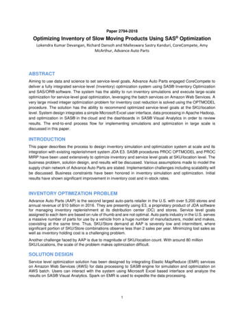
To optimize the service level goal at distribution center (DC) and stores, two independent simulations foreach SKU/Store and SKU/DC are designed. The following assumptions are made to model supply chainnetwork for Proc MIRP simulation.1. DC inventory simulation and store inventory simulations are independent. SKU/Store simulation isalso independent of other stores.2. SKU/Stores and SKU/DC forecast is used to model SKU demand in the MIRP simulation. Variance issame as daily mean demand as Poisson distribution is assumed.3. Simulation horizon 565 days and 200 days are used as warm up period.4. Margin is difference between retail price and current unit cost.Figure 1 below explains the process flow of the system designed.Figure 1 End to end process flowINVENTORY SIMULATION: SKU/LOCATIONInventory simulation is designed to observe how will the SKU/location behave for different values of servicelevel goals considering supply chain constraints like SKU demand and variance, lead time etc.SAS procedure MIRP (Multi Echelon Inventory Replenishment Plan) has been used for designinginventory simulation model. PROC MIRP can be executed with different modeling objective values tunedto different business objective. OPTPOLICY and PREDICTKPI have been used for Advance Auto Parts.OPTPOLICY is used to generate the optimal inventory policies and PREDICTKPI is used to compute theinventory performance metrics such average inventory, fill rate etc. Any supply chain network can beorganized in the structure required in PROC MIRP and can be used to compute the inventory controlparameters and performance metrics. PROC MIRP procedures requires four datasets as input in a specifiedstructure. Descriptions of three datasets required are provided below in Table 12

DatasetsDescriptionDemandDataTakes demand and variance at customer facing SKU/locationNodeDataTakes supply chain network parameters such as lead time, PBR,batch size etc. at SKU/location.ArcDataTakes predecessor and successor information for supply chainnetwork locationsInventoryDataThis is not required when objective is OPTPOLICY. It takesinventory policy control values which are output fromOPTPOLOCY and initial value of inventory.Table 1 Input datasets to PROC MIRPData for simulation have been prepared using E3 systems, Advance Store Replenishment (ASR) andAdvance Warehouse Replenishment (AWR) for inventory replenishment at stores and DC. To simulate theAAP supply chain network, parameters values are taken from ASR, and AWR tables which are listed in theTable 2 belowSimulation ParameterSource for store simulationSource for DC simulation1Mean DemandASRAWR2VarianceASRDC order variance3Lead timeASRAWR4Periods betweenreview(PBR)ASRAWR5Batch sizeASRAWR6OrderminASRAWRTable 2 Simulation data sourcesBelow is snippet of code, used for executing MIRP procedure for SKU/location for different level of servicelevel goal. This structure is modified for running simulations for thousands of SKU/Stores and SKU/DC onthe AWS batch. Each SKU/location is simulated for 565 periods (days). Number of replication used is 2000.Proc mirp nodedata work.nodedataarcdata work.arcdatademanddata work.demanddataout temp optpolicy outputpolicyparam integerdemandmodel discretereplications 2000cv2 yesforecastinterval 1horizon 565maxcv 1objective optpolicy;run;proc sql;create table optpolicy output asselect a.networkid,a.skuloc,3

a.period,a.*,case when period 1 then initial inventory else . end as amountfrom temp optpolicy output aorder by networked,skuloc,period;quit;Proc mirp nodedata work.nodedataarcdata work.arcdatademanddata work.demanddatainventorydata optpolicy outputout predictkpi outputpolicyparam integerdemandmodel discretereplications 2000cv2 yesforecastinterval 1horizon 565maxcv 1objective predictkpi;run;Independent simulations for SKU/store and SKU/DC at different service levels (81% to 99%) for 565 periods(day) were executed and developed a library of inventory performance metrics for each unique combinationof supply chain network parameters. Inventory performance metrics are listed below1.2.3.4.5.6.7.On hand MeanBacklog MeanOrder up to levelReorder levelSafety stockFill rateReady rateOutput of PROC MIRP with objective PREDICTKPI produces above measures at period level. We dropmeasures for the first 200 periods to account for impact of initial inventory in the system and rest are usedfor computing averages at SKU/Location level. We used a conservative warm-up period since the demandis low; in 200 days, many SKUs would see a demand of only 1 unit.SERVICE LEVEL OPTIMIZATION: SKU/LOCATIONOptimization model picks the service level which minimizes the sum of holding cost and shortage cost.Parameters used in the optimization are defined belowHolding cost: Holding cost is set by the user and can vary by department, item class and vary between DCand store.Shortage cost (1-Fill Rate) x annual demand x product margin, where margin is mode of retail price minuscurrent unit cost.Indicesi: index for item4

j: index for storek: index for service level at storeq: index for DCr: index for service level at DCDecision Variablesx: binary for item-store-SL allocationy: binary for item-DC-SL allocationConstantsTotal Cost Store : Holding cost Shortage cost at storeInv store: Average inventory at storeInv cost store: Inventory cost at storeTotal Cost DC : Holding cost Shortage Cost at DCInv DC: Average inventory at DCInv cost DC: Inventory cost at DC.Objective:Minimize: Total Cost (Holding Cost Shortage Cost) across all SKU-Stores and SKU-DCs (𝑥𝑖𝑗𝑘 Total Cost Store 𝑖𝑗𝑘 ) (𝑦𝑖𝑞𝑟 Total Cost DC 𝑖𝑞𝑟 )𝑖𝑖𝑘𝑖𝑞𝑟Decision:For each SKU-Store and SKU-DC, pick a ready rate. This is binary as only one Ready Rate can be picked.Thus, the number of binary variables will be equal to the sum of the number of ready-rate records acrossall SKU-Stores and SKU-DCs. We have defined two categories of binary decision variable 1. Store-SKUbinary and DC-SKU binary. Hence decision variables𝑥𝑖𝑗𝑘 and 𝑦𝑖𝑞𝑟 are binary variablesConstraints:Set 1: Store-SKU and DC-SKU can have only one Service Level. Pick only one ready rate. (ensures onlyone ready rate is selected for a SKU-Store or SKU-DCFor each SKU-store, sum of binaries 1 (𝑥𝑖𝑗𝑘 ) 1 𝑓𝑜𝑟 𝑖, 𝑗𝑘For each SKU-DC, sum of binaries 1 (𝑦𝑖𝑞𝑟 ) 1 𝑓𝑜𝑟 𝑖, 𝑞𝑟When there is no budget constraint model recommends optimum service level without taking account ofallocated budget. Note that since we are balancing holding cost and Shortage Cost, optimization will notpick the ready rate of 99% unless justified; the max ready rate might be incurring very high holding cost andnot giving us enough reduction in Shortage Cost.Set 2: Budget for inventory is limitedFor all SKU-Locations and their ready rates, total cost of inventory cannot exceed budgetInventory cost for SKU/Locations will be average inventory at given Ready Rate X Unit cost of the SKU 𝑥𝑖𝑗𝑘 Inv store𝑖𝑗𝑘 Inv cost store𝑖𝑗𝑘 𝑥𝑖𝑗𝑘 Inv DC𝑖𝑗𝑘 Inv cost DC𝑖𝑗𝑘𝑖𝑖𝑘𝑖𝑖𝑘 𝐵𝑢𝑑𝑔𝑒𝑡PROC OPTMODEL is used to model the above optimization problem which is executed on AWS cloudusing batch services.TECHNICAL CHALLENGES AND RESOLUTIONS5