Transcription
COREMetadata, citation and similar papers at core.ac.ukProvided by DSpace at VSB Technical University of OstravaKolkova, A. (2018). Indicators of Technical Analysis on the Basis of Moving Averages as PrognosticMethods in the Food Industry. Journal of Competitiveness, 10(4), 102–119. https://doi.org/10.7441/joc.2018.04.07INDICATORS OF TECHNICAL ANALYSIS ON THEBASIS OF MOVING AVERAGES AS PROGNOSTICMETHODS IN THE FOOD INDUSTRY Andrea KolkovaAbstractCompetitiveness is an important factor in a company’s ability to achieve success, and properforecasting can be a fundamental source of competitive advantage for an enterprise. The aimof this study is to show the possibility of using technical analysis indicators in forecasting pricesin the food industry in comparison with classical methods, namely exponential smoothing. Inthe food industry, competitiveness is also a key element of business. Competitiveness, however,requires not only a thorough historical analysis not only of but also forecasting. Forecastingmethods are very complex and are often prevented from wider application to increase competitiveness. The indicators of technical analysis meet the criteria of simplicity and can thereforebe a good way to increase competitiveness through proper forecasting. In this manuscript, theuse of simple forecasting tools is confirmed for the period of 2009-2018. The analysis was completed using data on the main raw materials of the food industry, namely wheat food, wheatforage, malting barley, milk, apples and potatoes, for which monthly data from January 2009 toFebruary 2018 was collected. The data file has been analyzed and modified, with an analysis ofindicators based on rolling averages selected. The indicators were compared using exponentialsmoothing forecasting. Accuracy RMSE and MAPE criteria were selected. The results showthat, while the use of indicators as a default setting is inappropriate in business economics, theiraccuracy is not as strong as the accuracy provided by exponential smoothing. In the followingsection, the models were optimized. With these optimized parameters, technical indicators seemto be an appropriate tool.Keywords: forecasting, technical indicator, exponential smoothing, simple average moving, exponential averagemoving, competitivenessJEL Classification: C53, G17, M21Received: May, 20181st Revision: October, 2018Accepted: November, 20181. INTRODUCTIONPrognosis is an integral part of corporate governance. Prognostic practice is currently applied using a wide range of different approaches and methods. Forecasting methods can be classified intwo ways. Qualitative methods include for example personal evaluation, panel match, the Delphi102joc4-2018-v2.indd 102Journal of Competitiveness1.12.2018 11:18:02
method, historical comparison, and market research. The second group consists of quantitativemethods, mostly reling on trending or causal models. In this paper, certain quantitative methodswill be applied, namely trend design.The importance of using quantitative methods in business was evidenced in a research by Wisniewski (1996), with the proportion of enterprises using quantitative methods found to be 66%. A rate of 24 % of companies indicated that the benefit of these methods is very high, while7 % of respondents in this research claimed no benefit. At this time, most business managers inenterprises applying quantitative methods used them to establish basic and descriptive statistics,cash flow discounting, quality control and inventory. Approximately 67 % of companies useddecision-making, compensation methods, with more than 50 % of such companies using simulations or regression analysis. Of course, it can be assumed that the use of quantitative methods inthe corporate economy has increased even more with the development of computing. With theproliferation of this technology, the number and complexity of the methods and models usedfor the prognosis of business variables have also increased. We can now make prognoses-basedpredictions using fuzzy logic, artificial neural networks, genetic algorithms, as well as chaostheory.The aim of this study is to show the possibility of using technical analysis indicators, a methodotherwise used predominantly for stocks, currencies and other financial assets, in predictingprices in the food industry in comparison with classical methods, namely exponential smoothing. This analysis examines accuracy based on ex-post forecasting.2. THEORETICAL BACKGROUNDThe history of prognosis is relatively short, dating only from the 1960s and early 1970s. The categorization as a separate scientific discipline is not unambiguous, and even the very definition ofprognosis has varied considerably since its inception.For example, Holcr (1981) defines prognosis as a form of a forecast which meets certain requirements, and it must contain the time or space interval in which the predicted phenomenon is orwill be discovered. The interval must be final, and there must be a principle possibility of an apriori estimation of the predicted phenomenon; the predicted phenomenon must be verifiableand, finally, the particular prognosis must be formulated completely accurately and unambiguously.Gál (1999) defines prognosis as a conditional statement about the future of an object or phenomenon based on scientific knowledge.According to Wishniewski (1996), the intention of prognosis is to reduce the uncertainty ofknowledge about the future and provide additional information to allow managers to assessalternative options in the context of future conditions as well as to evaluate the future consequences of current decisions.More modern approaches to forecasting then include the definition of the prognosis as a methodof transforming past experience into the expected future.To Vincur & Zajac, prognosis (2007, p. 12) is defined as a scientific discipline, the subject of103joc4-2018-v2.indd 1031.12.2018 11:18:02
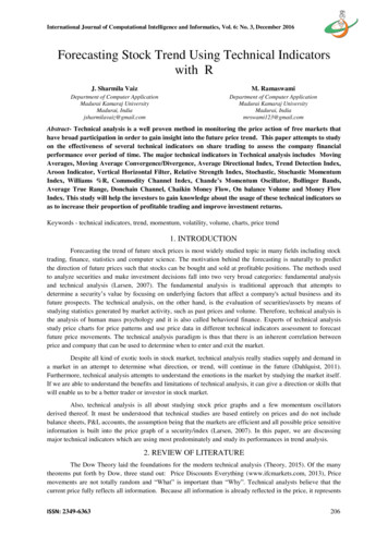
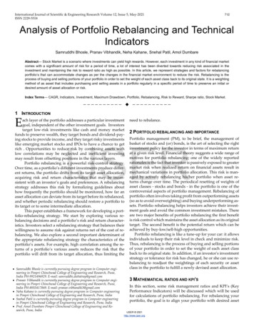
which is the study of the technical, scientific, economic and social factors and processes thatact on the development of the world’s objective reality and which aims to create a vision - theprognosis of a future condition resulting from the interconnected effects of these factors andprocesses.Forecasting methods can be broken down into several categories, with the most well-known andmost widely used divisions being within the general categories of qualitative and quantitativemethods. Miller & Swinehart (2010) categorized methods into three different groups: exploratory or normative methods, evidence-based methods, and assumptions based on evidence. Thethird grouping is then a classical breakdown into qualitative and quantitative methods. Moro etal. (2015) classify methods as quantitative, semi-quantitative and qualitative methods. Kesten &Armstrong (2014) divide forecasting methods into simple and complex forecasting along with awhole range of other subdivisions, as depicted in Figure riateSelfRoleStructuredSimulatedinteraction ompositionMultivariateDatabasedNo ExpertsystemsData ndexClassificationSegmentationFig. 1 – Methodolog y Tree of Forecasting. Source: Armstrong & Green, 2014.In this paper, the breakdowns set forth in Esmaelian et al. (2017) on quantitative, semi-quantitative and qualitative methods will be used.2.1 Qualitative forecastingQualitative methods usually do not duplicate numerical evaluations of data, but the professionalappreciation and verbal evaluation of the studied variables. These methods include, for example,an expert panel where a group of experts within a given organization study and discuss a givenquantity from different points of view (Wisnivski, 1996). Another method is the relevant tree(Daim et al, 2006), a way of identifying the development phases, objectives and basic elements104joc4-2018-v2.indd 104Journal of Competitiveness1.12.2018 11:18:02
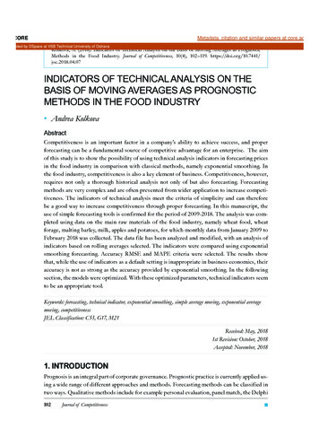
of a given enterprise quantity. A very similar method is the futures wheel, in which the event orquantity being investigated is considered the core of a wheel, and events or variables that canaffect it are considered to be vanes. A very well-known and used technique is the SWOT analysismethod, by which experts identify the strengths, weaknesses, opportunities and threats of thecompany or product. The literature review can also be considered another search method (Moroet al, 2015).2.2 Quantitative forecastingThese methods are usually based on mathematical-statistical techniques and numerical calculations, as indicated in Esmaelian et al. (2017). These include: trend analysis and trend extrapolation, which will be detailed in Chapter 3.1. Multi-stage analysis is a method that combines severalmodels, as defined along with other concepts by Antonic et al. (2011).We can also include the lesser known Future Workshop method by Martino (2003), as well assystem dynamics, a method that makes predictions based on dynamic tools such as neural networks, fuzzy logic, genetic algorithms, or chaos theory.In this paper, among the quantitative methods of forecasting, new methods of technical analysiswill be included as possible tools of forecasting in the corporate economy. These will be presented along with the trend analysis and trend extrapolation method, which explained in greaterdetail in Chapters 3.1 and 3.2.2.3 Semi-quantitative methodsSemi-quantitative methods include, for example, monitoring. This method uses systematic loopsto identify ideal conditions by means of feedback information. Another popular method is brainstorming, a process that collects a set of ideas about the future of an individual or a group ofpeople. Morphological analysis, questionnaire/surveys, scenario planning can also be characterized as this type of method.The Delphi method (Esmaelian, 2017), which uses questionnaires in consecutive rounds togather the views of as many experts as possible and to reach consensus, has also become popular. Also in wide use is stakeholder mapping (Saritas et al., 2013), (Vishnevskiy, 2015), a methodwhich uses statistical techniques to predict who the stakeholders are, where they are and whythey are interested in the product, bailout, etc. The text / data mining method used by, for example, Moro et al (2015), is one of the most recent techniques put into use.3. RESEARCH OBJECTIVE AND METHODOLOGYIn this paper, a prognosis regarding the evolution of selected prices in the food industry will bebased on historical prices and the ex-post forecast will be tested. The high prediction capabilityof the ex-post model is a prerequisite for using the ex-ante prognosis model. The ex-post relationship and the ex-ante prognosis are shown in Figure 2.105joc4-2018-v2.indd 1051.12.2018 11:18:02
Period of QuantificationParametrEstimation PeriodPeriod of ForecastingForecasting ex anteForecasting ex postTimePresenttimeFig. 2 – Time in Forecasting. Source: own according to Marček (2013), Vincúr (2007)Data for the main raw materials of the food industry, namely wheat food, wheat forage, maltingbarley, milk, apples and potatoes, has been analyzed. The data was obtained from the CzechStatistical Office from the monthly data collections from January 2009 to February 2018 in theCzech Republic. The data file has been analyzed and modified. Missing values were found regarding milk and potatoes and replaced by linear interpolation. Descriptive statistics of the dataare defined in Table 1.Tab. 1 – Descriptive Statistic of the Analyzed Data. Source: ownNMinMaxMeanStatisticSDVarianceSEStatisticwheat food110261261174214.0487.305915.662838436.090wheat ting ’s atoes1112159.0 16931.0 14493.0 9895.765126.89461336.91801787349.705The statistical programs SPSS and R (with TTR and FORECAST packages) were used for the analysis.3.1 Forecasts based on exponential equalizationFor this article, quantitative methods of forecasting based on exponential alignment were selected. Exponential smoothing is used for short-term forecasting in various modifications. Prognoses based on exponential smoothing consist of weighted averages of past values, with scalesexponentially decreasing with the age of the data used (Hyndman, 2018). Exponential alignmentmethods include simple exponential smoothing, Holt’s exponential smoothing and Winter’s exponential smoothing.As Bergmeir et al (2016) states, “the general idea of exponential smoothing is that recent observations are more relevant to forecasting than older observations, meaning that they should beweighted more highly.”joc4-2018-v2.indd 1061.12.2018 11:18:02
Simple exponential smoothing defines the prognosis as an exponential average and is used onlyfor non-periodic time series. The relationship of the extended equation has the Shape, ௧ܵ௧ ߙ σ௧ିଵ ୀ𝑖 (1 െ ߙ) ݕ ௧ିଵ (1 െ ߙ) ܵ , where(1)with T being the length of the time series, yt-1 the value of the time series, α (0, 1) the equaliza- ߚ ߚ(ܵ௧ െ ܵ௧ିଵ ) (1െ ߚ)ߚ(2)tionconstant,and S0 the initial equalizationvalue1,௧ିଵ , whereBrown’s multiple exponential smoothing defines the prognosis of polynomial trends with multiple exponential averages, which are obtained by another exponential equalization of alreadyobtained exponential averages. ܵ௧ െ ܵ௧ିଵ ߚ ,௧ െ ߚ ,௧ିଵHolt extended Brown’sexponentialsmoothingan adaptive estimation of(1)the trend compo (1(1 െ byܵ௧ ߙ σ௧ିଵߙ)௧௧ܵ , where௧ିଵ െ ߙ) ݕ ௧ିଵ (1 െ ߙ) ݕ ௧ିଵܵ௧ ߙ σ ୀ𝑖 (1 െ ߙ)(1) , where ୀ𝑖constantnent with the new balancingβ (Vincur& ܵZajac2007). The equalizationconstant canbe defined thusly,ߚ ߚ(ܵ௧ െ ܵ௧ିଵ ) (1 െ ߚ)ߚ 1,௧ିଵ , whereߚ ߚ(ܵ௧ െ ܵ௧ିଵ ) (1 െ ߚ)ߚ 1,௧ିଵ , where(2)(2) ܵ௧ െ ܵ௧ିଵ ߚ ,௧ െ ߚ ,௧ିଵ is the current state of trend and β1, t-1 is the adaptive estimate of the trendܵ௧ െ ܵ௧ିଵ ߚ ,௧ െ ߚ ,௧ିଵdirective over time. β is then the equalization constant. Holt’s double parametric linear exponential smoothing is a modification for the stochastic trend series.Damped trend methods have emerged as a response to the drawbacks of Holt linear methodsthat show a continuous trend. Empirical evidence, however, suggests that this can lead to excessive forecasts, especially in the longer forecast horizon. Methods of damped trends then includea parameter that dampens the trend on a straight line (Hyndman, 2018).There are currently several other methods summarized by Taylor (2003) as an additive dampedtrend method, multiplicative damped trend method, additive Holt-Winters method, multiplicative Holt-Winters method, Holt-Winters damped method.3.2 Forecasts based on technical analysis indicatorsThe objective of the technical analysis is to anticipate the future development of assets basedon an analysis of their past developments. Techniques based on technical indicators are alwaysbased on mathematical statistics. The technical analysis uses not only technical indicators, butalso graphical methods, with a more modern name of price action which are known even fromthe 18th century, when the Japanese applied their first candle charts to their rice deals. Today,they are published slightly less than technical indicators such as Lee & Jo (1999), and are thesubject of research rather based on programming.There are a lot of technical indicators. Back in 1988, Colby published an encyclopedia of technical market indicators (Colby, 2003). George Lane published his Lane’s stochastic oscillator morethan three decades ago (Lane, 1984), or even in the 1970s, the relative strength developed byWilder (1978). In the 80s-90s of the 20th century, indicators belonging to a group of channel systems were published, for Bollinger bands, John Bollinger (Bollinger, 1992), or Kaufman (1987).Of the newer indicators, for example, the Chaikin oscillator is known (Achelis, 2001) or todaythe most widely used MACD indicator introduced by Appel (2005). In 2007 (Cheung & Kaymak, 2007), a concept combining technical indicators and fuzzy logic was introduced. Abbasi107joc4-2018-v2.indd 1071.12.2018 11:18:02
and Abouec also used a system derived from neuro-fuzzy logic (Abbasi & Abouec, 2008). In2009, Chavarnakul & Enke, (2009) developed a hybrid exchange trading model using the Neurofuzzy concept called the Genetic Algorithm (NF-GA). In 2015, technical indicators (specificallyMACD and the lesser-known Gann-Hilo indicator) and fuzzy logic were used again (Chourmouziadis & Chatzoglou, 2015). Currently, there are still new indicators based on both fuzzymodeling and a combination of individual statistical and mathematical indicators, and so the listof indicators is far from complete. The existing ones are then subjected to various tests (da Costa,2015; Kolkova, 2017; Kresta, 2015).In this study, an innovative attempt is made to apply technical indicators to business economyphenomena as well. Technical analysis indicators have not yet been used to predict the businesseconomy and are not yet part of any research work, so their use can be a tool to significantly increase the competitiveness of the business. For the sake of scale, only some technical indicatorshave been selected, namely indicators on the basis of rolling averages, which are also one of themost used in the practice of financial transactions. Since the exponential equalization method isalso based on the methodological basis of moving averages, it can be assumed that these indicators may also be an appropriate tool for predicting business phenomena.Sliding averages calculate the average value of the data in the width of its timeframe. For example, a 7-day moving average means the average value of the last week, 14 days in the last twoweeks. After joining the rolling average of all days, we create a rolling average curve.The moving average is now a whole range. The basis is Simple Moving Average (SMA) and canbe defined by the relationship,ܵ ܣܯ σಿభ ௨௧𝑛𝑛, where(3)N is the number of days for which the SMA is numbered. Moving averages are used to smooth ି𝐸𝐸𝐸𝐸ܧ 𝐸𝐸𝐸𝐸ܧ ଵ ܭ ή (݅݊ ݐݑ െ ି𝐸𝐸𝐸𝐸ܧ ଵ ), or(4)arrayto help, eliminatenoise and identifytrends. The simple moving average is 𝐸𝐸𝐸𝐸ܧ the ܭ ή data݅݊ ݐݑ in an(1 െ 𝐸𝐸𝐸𝐸ܧ )ܭ (5)ିଵ whereliterally2 the simplest form of a moving average. Each output value is the average of the previous n, where(6)KN In1 a simple moving average, each value in the time period carries equal weight, and valuesvalues.outside of the time period are not included in the average. This makes it less responsive to recentchanges in െthedata, which can be useful for filtering ))ݐݑ ݊݅(𝐸𝐸𝐸𝐸ܧ(𝐸𝐸𝐸𝐸ܧ (7)out those changes. 𝐷𝐷𝐷𝐷𝐷𝐷ܦ 2 )ݐݑ ݊݅(𝐸𝐸𝐸𝐸ܧ Exponential moving average (EMA) is considered to be a better tool than a simple movingܼ ܭ 𝑍𝑍𝑍𝑍𝑍𝑍ܮ ή average൫2 ݅݊ (ݐݑ Elder,(1 െ )ܭ it ܼ 𝑍𝑍𝑍𝑍𝑍𝑍ܮ where weight(8)2006)becauseattachesto current data and changes in price െ ݅݊ ݐݑ ି ൯ ିଵ ,greater𝑛𝑛𝑛𝑛σಿభ. ௨௧݈ܽ݃ countlesstechnical indicators. It can beܵ ܣܯ , where(3)ଶ𝑛𝑛expressed by the relationship,ଵ௦𝑠𝑠 σ 𝐸𝐸𝐸𝐸ܧ 𝑠𝑠𝑠)(݀𝑑𝑑݂݂ ି𝐸𝐸𝐸𝐸ܧ ଵ 𝑡𝑡𝑡𝑡𝑡 )ܭ ,ή where(݅݊ ݐݑ െ ି𝐸𝐸𝐸𝐸ܧ ଵ ), or ୀ𝑖 ( ݏ ܭ 𝐸𝐸𝐸𝐸ܧ ή 𝑛𝑛݅݊ ݐݑ (1 െ ି𝐸𝐸𝐸𝐸ܧ )ܭ ଵ , where݉ ቔ ቕ,2, whereK ଶ ݏ උξN𝑛𝑛ඏ, 1ଵ 𝑚𝑚𝑓𝑓𝑓𝑓 𝑡𝑡𝑓𝑓𝑓𝑓ݎ σೞ σ ୀ𝑖 (݉ 𝑡𝑡𝑡 ), 𝑡𝑡𝐻𝐻𝐻𝐻ܪ σೞ స𝑖 N స𝑖is the number of days to quantify the EMA.ଵ 𝑠𝑠𝑠𝑠 ܿ݁ݏ σ𝑛𝑛𝑛𝑛െ ))ݐݑ ݊݅(𝐸𝐸𝐸𝐸ܧ(𝐸𝐸𝐸𝐸ܧ 𝑡𝑡𝐷𝐷𝐷𝐷𝐷𝐷ܦ σ2ೞ )ݐݑ ݊݅(𝐸𝐸𝐸𝐸ܧ 𝑡𝑡𝑡𝑡𝑡 ), ୀ𝑖 (𝑛𝑛𝑛𝑛𝑛)(݅݊ ݐݑ (10)(11)(12)(13)(14)(4)(5)(6)(7) స𝑖Doubleexponential moving average (hereafter DEMA), as reported by FM Labs (2016), is a݀𝑑𝑑݂݂𝑡𝑡 2 𝑓𝑓𝑓𝑓 𝑡𝑡𝑓𝑓𝑓𝑓ݎ െ 𝑡𝑡𝑠𝑠𝑠𝑠 ܿ݁ݏ , or(15)smoothing indicator less lag than straight EMA. It is more complex than just moving average.𝑛𝑛 ݅݊ ݐݑ െ ݅݊ ିݐݑ ൯ (1 െ ି𝑍𝑍𝑍𝑍𝑍𝑍ܮܼ )ܭ ଵ , where (8)ܼ 𝑍𝑍𝑍𝑍𝑍𝑍ܮ DEMA ܭ ή ൫2wasdevelopedby Mulloy(1994). It can be(16)defined by the relationship, (𝑊𝑊𝑊𝑊ܹ 𝐻𝐻𝐻𝐻ܪ 2 ܹ𝑊𝑊𝑊𝑊െ ܹ𝑊𝑊𝑊𝑊(𝑛𝑛), ))𝑛𝑛(𝑠𝑠𝑠𝑠ݍݏ ,where108ଵ𝐴𝐴𝐴𝐴𝐴𝐴𝐴𝐴 ேைோெଵ 𝑡𝑡𝐻𝐻𝐻𝐻ܪ σೞ స𝑖 𝑛𝑛𝑛𝑛ଶ݈ܽ݃ .ଶJournal of ିCompetitiveness( ష 𝑜𝑜 )మ మσ௦𝑠𝑠௭ , where ୀ𝑖 𝑝𝑝(݅)𝑒𝑒 σ௦𝑠𝑠 ୀ𝑖 ( ݏ �𝑡 ), where𝑛𝑛݉ ቔσಿ 𝑝𝑝ቕ, ௬ ି௬ෞ ൯మܴଶ ଶಿమ,ത൯ 𝑝𝑝 ௬ ି௬ ݏ උξσ𝑛𝑛ඏ,(10)orమjoc4-2018-v2.indd 108 ଶ ଵσಿ 𝑝𝑝 𝑒𝑒 1െ σ 𝑚𝑚(݉ 𝑓𝑓 ܴ 𝑓𝑓𝑓𝑓ݎ .(18)),(19)(11)(12)(13)1.12.2018 11:18:03
ܵ ܣܯ భ ௨௧𝑛𝑛, where(3) ି𝐸𝐸𝐸𝐸ܧ 𝐸𝐸𝐸𝐸ܧ ଵ ܭ ή (݅݊ ݐݑ െ ି𝐸𝐸𝐸𝐸ܧ ଵ ), orσಿ ௨௧ െ 𝐸𝐸𝐸𝐸ܧ )ܭ ܭ ή ݅݊ ݐݑ ܣܯܵ 𝐸𝐸𝐸𝐸ܧ ିଵ , where భ (1, whereK(4)(5)(3)(6)2 𝑛𝑛, whereN 1σಿ ௨௧ܵ ܣܯ భ ܭ ή (݅݊ ݐݑ , where(3) 𝐸𝐸𝐸𝐸ܧ 𝐸𝐸𝐸𝐸ܧ െ ି𝐸𝐸𝐸𝐸ܧ ଵ ), or(4)𝑛𝑛ିଵ(5) ܭ 𝐸𝐸𝐸𝐸ܧ ή ݅݊ ݐݑ (1 െ ି𝐸𝐸𝐸𝐸ܧ )ܭ ଵ , whereെ ))ݐݑ ݊݅(𝐸𝐸𝐸𝐸ܧ(𝐸𝐸𝐸𝐸ܧ (7) 𝐷𝐷𝐷𝐷𝐷𝐷ܦ 2 )ݐݑ ݊݅(𝐸𝐸𝐸𝐸ܧ 2, where(6)K 𝐸𝐸𝐸𝐸ܧ 𝐸𝐸𝐸𝐸ܧ ܭ ή(݅݊ ݐݑ െ 𝐸𝐸𝐸𝐸ܧ ),or(4) This indicator was createdN ିଵ1ିଵ is a variation of the EMA.The Zero-Lag exponentialmoving average(5) ܭ 𝐸𝐸𝐸𝐸ܧ ή ݅݊ ݐݑ (1 െ ି𝐸𝐸𝐸𝐸ܧ )ܭ ଵ , whereܼ 𝑍𝑍𝑍𝑍𝑍𝑍ܮ ܭ ൫2 ݅݊ ݐݑ ݅݊ ݐݑ (1benefitെ 𝑍𝑍𝑍𝑍𝑍𝑍ܮܼ )ܭ , whereweighting(8)byEhlers&ή Way(2010)keepsof the ିଵheavierof recent values but atି ൯ the2 െand, where(6)𝑛𝑛𝑛𝑛K.(9)tempts to2removelagby older data to minimize the cumulativeeffect. It is expressedN݈ܽ݃ 1 )ݐݑ ݊݅(𝐸𝐸𝐸𝐸ܧ െsubtracting ))ݐݑ ݊݅(𝐸𝐸𝐸𝐸ܧ(𝐸𝐸𝐸𝐸ܧ (7) 𝐷𝐷𝐷𝐷𝐷𝐷ܦ ଶσಿ ௨௧by the relationship,ܵ ܣܯ భ, where(3)𝑛𝑛ଵ ܭ ௦𝑠𝑠2 )ݐݑ ݊݅(𝐸𝐸𝐸𝐸ܧ െ ))ݐݑ ݊݅(𝐸𝐸𝐸𝐸ܧ(𝐸𝐸𝐸𝐸ܧ (7) 𝐷𝐷𝐷𝐷𝐷𝐷ܦ ܼ 𝑍𝑍𝑍𝑍𝑍𝑍ܮ ή൫2 ݅݊ ݐݑ െ݅݊ ݐݑ ൯ (1െ )ܭ ܼ 𝑍𝑍𝑍𝑍𝑍𝑍ܮ ,where(8) ିଵ 𝑡𝑡𝐻𝐻𝐻𝐻ܪ σೞ σ ୀ𝑖 ( ݂݂𝑑𝑑݀()𝑠𝑠𝑠 ݏ ), where(10)𝑡𝑡𝑡𝑡𝑡ି 𝑛𝑛𝑛𝑛 స𝑖 ݈ܽ݃ 𝑛𝑛 .(9)(4) (11) ି𝐸𝐸𝐸𝐸ܧ 𝐸𝐸𝐸𝐸ܧ ଵ ݉ܭ ή (݅݊ ݐݑ ቔ ቕ,ଶ െ ି𝐸𝐸𝐸𝐸ܧ ଵ ), orଶ ܭ ή݅݊ ݐݑ (1 𝐸𝐸𝐸𝐸ܧ (5) Alan 𝐸𝐸𝐸𝐸ܧ ܼ 𝑍𝑍𝑍𝑍𝑍𝑍ܮ ܭ ή൫2 ݅݊ ݐݑ െ൯, where HMA),(1 െ )ܭ developedܼ ି𝑍𝑍𝑍𝑍𝑍𝑍ܮ ଵ , where(8)Hull (2012), is an improvedିଵ ξ )ܭ ି Hull moving averageonlyby ݏ െඋ(hereafter𝑛𝑛ඏ,݅݊ ݐݑ (12)𝑛𝑛𝑛𝑛2 ଵଵ 𝑚𝑚݈ܽ݃ .(9),where(6)K 𝑡𝑡the௦𝑠𝑠 σ average,𝑓𝑓𝑓𝑓 𝑓𝑓𝑓𝑓ݎ ),(13) reversal quite accurately. It isvariantshowsthe moment of trend 𝐻𝐻𝐻𝐻ܪ , where𝑡𝑡𝑡𝑡𝑡(10)ೞ1 ( ݂݂𝑑𝑑݀()𝑠𝑠𝑠 ݏ ୀ𝑖 ��𝑡 of𝑡𝑡𝑡𝑡𝑡 )whichೞ ୀ𝑖Nσ σmoving స𝑖 σ స𝑖 ଵ𝑛𝑛 (𝑛𝑛𝑛𝑛𝑛)(݅݊ ݐݑ definedby therelationship, 𝑠𝑠𝑠𝑠 ܿ݁ݏ σቔ𝑛𝑛𝑛𝑛𝑡𝑡 ೞ ݉ 𝑡𝑡𝑡𝑡𝑡 ),ቕ, ୀ𝑖σ స𝑖 ଵଶ σ௦𝑠𝑠𝑠𝑠𝑠)(݀𝑑𝑑݂݂), where݀𝑑𝑑݂݂2 ))ݐݑ ݊݅(𝐸𝐸𝐸𝐸ܧ(𝐸𝐸𝐸𝐸ܧ උ𝑓𝑓𝑓𝑓 𝑓𝑓𝑓𝑓ݎ 𝑠𝑠𝑠𝑠 ܿ݁ݏ ݏ(ݏ 𝑡𝑡 𝑡𝑡 , orξ𝑛𝑛ඏ, 𝑡𝑡 െ𝑡𝑡𝑡𝑡𝑡 ୀ𝑖 𝐻𝐻𝐻𝐻ܪ𝐷𝐷𝐷𝐷𝐷𝐷ܦ 2𝑡𝑡 )ݐݑ ݊݅(𝐸𝐸𝐸𝐸ܧ െ σೞ స𝑖 ଵ𝑛𝑛 𝑚𝑚𝑚)(݅݊𝑝𝑝𝑝𝑝𝑝𝑝σ 𝑚𝑚(݉𝑓𝑓𝑓𝑓 𝑡𝑡𝑓𝑓𝑓𝑓ݎ σೞ ݉𝑡𝑡𝑡𝑡𝑡 ), ୀ𝑖𝑛𝑛 െቔ ܹ𝑊𝑊𝑊𝑊(𝑛𝑛),ቕ, ܹ𝑊𝑊𝑊𝑊 ))𝑛𝑛(𝑠𝑠𝑠𝑠ݍݏ , where (𝑊𝑊𝑊𝑊ܹ 𝐻𝐻𝐻𝐻ܪ 2 స𝑖ଶଵଶ 𝑛𝑛𝑛𝑛σ ୀ𝑖 (𝑛𝑛𝑛𝑛𝑛)(݅݊ 𝑍𝑍𝑍𝑍𝑍𝑍ܮܼ) 𝑡𝑡𝑡𝑡𝑡ݐݑ ,උξ𝑛𝑛ඏ,𝑡𝑡 σ ೞ െ ݏ ή ൫2 ݅݊ ݐݑ ܼ 𝑠𝑠𝑠𝑠 ܿ݁ݏܭ 𝑍𝑍𝑍𝑍𝑍𝑍ܮ ݅݊ ݐݑ ି ൯ (1 െ )ܭ ିଵ , whereଵ స𝑖 𝑛𝑛𝑛𝑛 𝑚𝑚( ష 𝑜𝑜 )మσ𝑓𝑓𝑓𝑓 ݂݂𝑑𝑑݀𝑡𝑡𝑓𝑓𝑓𝑓ݎ ݈ܽ݃ (݉𝑚𝑚𝑚)(݅݊𝑝𝑝𝑝𝑝𝑝𝑝)ଵ2 ୀ𝑖𝑓𝑓𝑓𝑓 𝑓𝑓𝑓𝑓ݎ െି 𝑠𝑠𝑠𝑠 ܿ݁ݏ , 𝑡𝑡𝑡𝑡𝑡or ,ೞ ௦𝑠𝑠௭ .𝑡𝑡𝑡𝑡𝑡𝑡మσ σ𝐴𝐴𝐴𝐴𝐴𝐴𝐴𝐴 స𝑖 ୀ𝑖, whereଶ 𝑝𝑝(݅)𝑒𝑒ேைோெଵ 𝑡𝑡𝑠𝑠𝑠𝑠 ܿ݁ݏ σೞ 𝑛𝑛 σ𝑛𝑛𝑛𝑛 ୀ𝑖 (𝑛𝑛𝑛𝑛𝑛)(݅݊ ) 𝑡𝑡𝑡𝑡𝑡ݐݑ , (𝑊𝑊𝑊𝑊ܹ 𝐻𝐻𝐻𝐻ܪ 2 ܹ𝑊𝑊𝑊𝑊 స𝑖 െ ܹ𝑊𝑊𝑊𝑊(𝑛𝑛), ))𝑛𝑛(𝑠𝑠𝑠𝑠ݍݏ , where݀𝑑𝑑݂݂𝑡𝑡 2ଶ 𝑓𝑓𝑓𝑓 𝑡𝑡𝑓𝑓𝑓𝑓ݎ െ 𝑡𝑡𝑠𝑠𝑠𝑠 ܿ݁ݏ , orଵమ 𝑡𝑡𝐻𝐻𝐻𝐻ܪ σೞ σ௦𝑠𝑠( ݂݂𝑑𝑑݀()𝑠𝑠𝑠 ݏ σಿෞ ൯𝑡𝑡𝑡𝑡𝑡 )ଶ, where ୀ𝑖 𝑝𝑝 ௬ ି௬( ష 𝑜𝑜 )మ స𝑖 మ , orଵି σಿ మ𝑛𝑛 ܴ ௦𝑠𝑠௭ 𝑛𝑛 ௬ ݉ 𝑝𝑝(݅)𝑒𝑒,ത൯where where ି௬ 𝑝𝑝 𝐴𝐴𝐴𝐴𝐴𝐴𝐴𝐴 𝐻𝐻𝐻𝐻ܪ ܹ𝑊𝑊𝑊𝑊(2 ܹ𝑊𝑊𝑊𝑊ܹ𝑊𝑊𝑊𝑊(𝑛𝑛), ))𝑛𝑛(𝑠𝑠𝑠𝑠ݍݏ ,ቔ σቕ, ୀ𝑖ଶ െேைோெమଶσಿ 𝑝𝑝 𝑒𝑒 ଶܴ 1െ.మ ݏ උξ𝑛𝑛ඏ,ಿσ 𝑝𝑝( ష 𝑜𝑜 )WMA is weightedmoving average. ௬ ି௬ത൯ మଵଵି మమσ௦𝑠𝑠௭ 𝐴𝐴𝐴𝐴𝐴𝐴𝐴𝐴 𝑝𝑝(݅)𝑒𝑒σಿ 𝑡𝑡𝑡𝑡𝑡𝑓𝑓𝑓𝑓 𝑡𝑡𝑓𝑓𝑓𝑓ݎ σ ೞ ୀ𝑖 ୀ𝑖 (݉ෞ,൯ where ௬),ି௬(14)(11)(10)(12)(7) (15)(13)(11)(16)(14)(12)(8)(13)(9) (15)(17)(14)(16)(15)(10)(18)(16)(11) (17)(19)(12)(13)(17) ேைோெ 𝑝𝑝 ଶ స𝑖 ଶ మ , or ALMA) by the authorsArnaud σLegouxmovingଵܴaverage ಿ (hereafter(18) Legoux & Kouzis-Loukasଵ𝑛𝑛𝑛𝑛 σேെ ݕ ෞ൯ ௬𝑝𝑝 )ି௬𝑝𝑝𝑝𝑝𝑝ା𝑝 𝑝𝑝ݕ σ 𝑝𝑝 𝑡𝑡𝑠𝑠𝑠𝑠 ܿ݁ݏ σೞ𝑀𝑀𝑀𝑀𝑀𝑀 σ (𝑛𝑛𝑛𝑛𝑛)(݅݊ ݐݑ , .ത൯(14) (20)𝑀𝑀𝑡𝑡𝑡𝑡𝑡 ୀ𝑖ಿ 𝑒𝑒 మuses the curvedistributionwhichcanbeplaced by offset parameter from స𝑖 of the normalσ(Gauss) మܴଶ 1 𝑠𝑠𝑠𝑠 ܿ݁ݏ െ ಿ 𝑝𝑝 2 𝑓𝑓𝑓𝑓 𝑓𝑓𝑓𝑓ݎ െ, ି௬or ௬(15) (19)మ. ෞ ൯σ𝑡𝑡ಿ𝑡𝑡 allows the smoothness and high sensitivity of the moving aver 𝑝𝑝ത൯ ି௬ ௬0 to 1. ݀𝑑𝑑݂݂This𝑡𝑡 parameterregulating 𝑝𝑝ܴ𝑅𝑅𝑅𝑅𝑅𝑅 ܴଶσξ𝑀𝑀𝑀𝑀𝑀𝑀.(21) ಿ(18)మ , orσ 𝑝𝑝 ௬ ି௬ത൯𝑛𝑛Sigmais anotherparameterresponsible for the(16)shape of the curve coefficients. Thisಿ thatమଶ is 𝐻𝐻𝐻𝐻ܪ age.ܹ𝑊𝑊𝑊𝑊(2 ܹ𝑊𝑊𝑊𝑊െ ଵܹ𝑊𝑊𝑊𝑊(𝑛𝑛), ))𝑛𝑛(𝑠𝑠𝑠𝑠ݍݏ ,whereσ𝑒𝑒ଵ 𝑝𝑝ேே𝑀𝑀𝑀𝑀𝑀𝑀 ܴଶσσ ݕ െ ݕ ෞ൯.మ.𝑀𝑀𝑀𝑀𝑀𝑀ଶreducesห ݕ ಿ𝑝𝑝𝑝𝑝ofെthe ݕ ෞห(22)1a െ(19)𝑝𝑝𝑝𝑝 .information𝑝𝑝𝑝𝑝𝑝ା𝑝moving averagelagbut still being(20)smoothto reduce noises.𝑀𝑀𝑀𝑀 𝑝𝑝𝑝𝑝𝑝ା𝑝σ 𝑝𝑝 ௬ത൯ ି௬𝐴𝐴𝐴𝐴𝐴𝐴𝐴𝐴 ଵ( ష 𝑜𝑜 )మିଶ మσ௦𝑠𝑠௭ 𝑝𝑝(݅)𝑒𝑒ෞ หห௬ଶ ି௬ଵ ே , where ୀ𝑖 ܴ𝑅𝑅𝑅𝑅𝑅𝑅ଵ ே ξ𝑀𝑀𝑀𝑀𝑀𝑀.σ െ ݕ ݕ 𝑀 𝑀𝑀𝑀𝑀ܲ𝑀𝑀ෞ൯ .𝑀𝑀 𝑝𝑝𝑝𝑝𝑝𝑝𝑝ା𝑝𝑝𝑝 ௬ேைோெ𝑀𝑀ଵ ேσห 𝑝𝑝ݕ െ ݕ ෞห𝑝𝑝 .𝑀𝑀 𝑝𝑝𝑝𝑝𝑝ା𝑝మಿ ���σ ෞ ൯ 𝑝𝑝 ௬ ି௬ଶsize is the window size.𝑀𝑀𝑀𝑀𝑀𝑀 ܴ σି௬ത൯ଵ ௬ 3.3 Forecasting 𝑀𝑀𝑀𝑀ܲ𝑀𝑀accuracyଵ ே 𝑝𝑝ಿσమ ே ಿమ, or ଶෞ หห௬ ି௬(17) ��� σ𝑝𝑝𝑝𝑝𝑝ା𝑝ෞห(22)σ 𝑝𝑝𝑀𝑀𝑒𝑒 ห 𝑝𝑝𝑝𝑝𝑝ݕ ା𝑝𝑝𝑝 െ ݕ 𝑝𝑝 . ௬ 𝑀𝑀ܴଶto predict1െ(19)models, it is advisable to choose theమ.If it is possibleby multiple methods orಿ the valuesσ 𝑝𝑝 ௬ ି௬ത൯ଶone that provides the smallesterrors.ห௬ Theෞ ห error rate should be evaluated at the time of knownି௬ଵ ே.(23)ଵ ே 𝑀𝑀𝑀𝑀ܲ𝑀𝑀 𝑀𝑀 σଶ𝑝𝑝𝑝𝑝𝑝ା𝑝௬ σ ݕ െ ݕ ෞ൯(20)then, if the chosen error estimatingvalues 𝑀𝑀𝑀𝑀𝑀𝑀in the ex-postforecasting𝑝𝑝 . period. For the evaluation𝑀𝑀 𝑝𝑝𝑝𝑝𝑝ା𝑝 𝑝𝑝variable is 0 then the prognosis is flawless. In the case of a positive error, the model underesܴ𝑅𝑅𝑅𝑅𝑅𝑅 ξ𝑀𝑀𝑀𝑀𝑀𝑀.(21)timates the fact,and vice versa, in the case of a negativemodel error, the fact overestimatesଵ ே root mean square error (hereafter RMSE), mean absolute percentage errorthe fact.R-squared,𝑀𝑀𝑀𝑀𝑀𝑀 σ𝑝𝑝𝑝𝑝𝑝ା𝑝ห 𝑝𝑝ݕ െ ݕ ෞห(22)𝑝𝑝 .𝑀𝑀(hereafter MAPE), maximum absolute perceived error (hereafter MaxAPE), mean absolute erଶෞ หห௬ absoluteି௬ଵror ror (hereafter (23)MaxAE) and the normalized Bayesian σே.𝑀𝑀 𝑝𝑝𝑝𝑝𝑝ା𝑝௬ information criterion (hereafter Normalized BIC) are used as prognostic accuracy measures.The formulas in this article were drawn mainly from (Vincur & Zajac, 2007) and (Marček, 2013).R-squared is usually called the coefficient of determination. It is the proportion of variation invariable explained by the model,109joc4-2018-v2.indd 1091.12.2018 11:18:04
σ ೞ݅݊ ݐݑ σσ ௨௧(𝑛𝑛𝑛𝑛𝑛)(݅݊ ݐݑ ), ି𝑍𝑍𝑍𝑍𝑍𝑍ܮܼ )ܭ ଵ , where (14) 𝑠𝑠𝑠𝑠 ܿ݁ݏ 𝑡𝑡𝑡𝑡𝑡െܼ 𝑍𝑍𝑍𝑍𝑍𝑍ܮ σ ܭ స𝑖𝑡𝑡ή ൫2െ ݅݊ ݐݑ (8)݈ܽ݃ ି ൯. (1ܵ ܣܯ భ ୀ𝑖, where(3) స𝑖ଶ݀𝑑𝑑݂݂𝑡𝑡 2 𝑓𝑓𝑓𝑓 𝑓𝑓𝑓𝑓ݎ (15)𝑛𝑛𝑛𝑛 𝑡𝑡 , or𝑡𝑡 െ𝑛𝑛 𝑠𝑠𝑠𝑠 ܿ݁ݏ ݀𝑑𝑑݂݂ 2 𝑓𝑓𝑓𝑓 𝑓𝑓𝑓𝑓ݎ െ 𝑠𝑠𝑠𝑠 ܿ݁ݏ ,or(15)݈ܽ݃ .(9)𝑡𝑡𝑡𝑡െ ))ݐݑ ݊݅(𝐸𝐸𝐸𝐸ܧ(𝐸𝐸𝐸𝐸ܧ 𝐷𝐷𝐷𝐷𝐷𝐷ܦ 2𝑡𝑡 )ݐݑ ݊݅(𝐸𝐸𝐸𝐸ܧ ଶ𝑛𝑛(9)(7)𝑛𝑛 ܹ𝑊𝑊𝑊𝑊(2 ܹ𝑊𝑊𝑊𝑊 ଵെ ܹ𝑊𝑊𝑊𝑊(𝑛𝑛), ))𝑛𝑛(𝑠𝑠𝑠𝑠ݍݏ , where(16) 𝐻𝐻𝐻𝐻ܪ 𝐻𝐻𝐻𝐻ܪ ܹ𝑊𝑊𝑊𝑊(2 ଶೞܹ𝑊𝑊𝑊𝑊(16)σ௦𝑠𝑠 𝐸𝐸𝐸𝐸ܧ σ 𝐸𝐸𝐸𝐸ܧ െ ܭ ή 𝑠𝑠𝑠)(݀𝑑𝑑݂݂(݅݊ ݐݑ െ ))𝑛𝑛(𝑠𝑠𝑠𝑠ݍݏ , 𝐸𝐸𝐸𝐸ܧ or(4) (10) ିଵ( )𝑛𝑛(𝑊𝑊𝑊𝑊ܹݏ ,), whereିଵ ),where𝑡𝑡 𝑡𝑡𝑡𝑡𝑡 ୀ𝑖ଶ స𝑖 ଵ ܭ ௦𝑠𝑠ή ݅݊ ݐݑ (1െ )ܭ 𝐸𝐸𝐸𝐸ܧ 𝐸𝐸𝐸𝐸ܧ ,where(5) ܭ ή൫2 ݅݊ ݐݑ െ݅݊ ݐݑ ൯ (1െ )ܭ ܼ 𝑍𝑍𝑍𝑍𝑍𝑍ܮ ,where(8)ିଵ𝑛𝑛σమ ( ݏ 𝑠𝑠𝑠)(݀𝑑𝑑݂݂),where(10) 𝑍𝑍𝑍𝑍𝑍𝑍ܮܼ 𝑡𝑡𝐻𝐻𝐻𝐻ܪ ି ିଵ( ష 𝑜𝑜 )𝑡𝑡𝑡𝑡𝑡 ቕ, ୀ𝑖σೞ ଵ (11)మ2 ି ݉ మ ቔ( ష 𝑜𝑜 )ଶ ,𝑛𝑛𝑛𝑛ଵ �� స𝑖 σK௦𝑠𝑠௭ where(17)ି ௦𝑠𝑠௭ ,where(6) ୀ𝑖మ݈ܽ݃.(9)𝑛𝑛 ேைோெ σ ୀ𝑖𝐴𝐴𝐴𝐴𝐴𝐴𝐴𝐴, where(17) (11) (12)N݉1 ቔ𝑝𝑝(݅)𝑒𝑒 ݏ ቕ, උξ𝑛𝑛ඏ,ଶேைோெଶଵσ 𝑚𝑚 ݏ ೞ උξ𝑛𝑛ඏ,(12) (13)𝑓𝑓𝑓𝑓 𝑡𝑡𝑓𝑓𝑓𝑓ݎ �𝑡𝑡𝑡𝑡 ୀ𝑖σ స𝑖 మಿ ௬ ି௬ 𝑚𝑚ଵଵ σ௦𝑠𝑠σෞ൯ଵమ 𝑝𝑝 )𝑓𝑓𝑓𝑓 𝑓𝑓𝑓𝑓ݎ ଶ ୀ𝑖 ( ݏ 𝐻𝐻𝐻𝐻ܪ 𝑡𝑡 σ)𝑡𝑡𝑡𝑡𝑡σಿෞି௬ 2𝑡𝑡𝑡𝑡 )ݐݑ ݊݅(𝐸𝐸𝐸𝐸ܧ ))ݐݑ ݊݅(𝐸𝐸𝐸𝐸ܧ(𝐸𝐸𝐸𝐸ܧ (7) (10) 𝐷𝐷𝐷𝐷𝐷𝐷ܦ σ𝑛𝑛𝑛𝑛(𝑛𝑛𝑛𝑛𝑛)(݅݊ ݐݑ (14) 𝑠𝑠𝑠𝑠 ܿ݁ݏ σೞೞ స𝑖 ܴ σೞ െಿ ଶ𝑠𝑠𝑠)(݀𝑑𝑑݂݂, 𝑡𝑡𝑡𝑡𝑡(18) ୀ𝑖 or , ൯where 𝑡𝑡𝑡𝑡𝑡 ), 𝑝𝑝మ ௬ ୀ𝑖σ స𝑖(18)σܴത൯ ௬ ି௬ స𝑖మ , or 𝑝𝑝 ଵσಿ ௬ ି௬ത൯ ),𝑛𝑛 𝑝𝑝 𝑡𝑡𝑠𝑠𝑠𝑠 ܿ݁ݏ σೞ ݀𝑑𝑑݂݂ (݅݊ ݐݑ (14)ಿమ𝑡𝑡𝑡𝑡𝑡 ݉2𝑒𝑒 (15) ୀ𝑖ቔ ቕ, 𝑡𝑡 మെ 𝑠𝑠𝑠𝑠 ܿ݁ݏ (11)𝑡𝑡 , or 𝑓𝑓𝑓𝑓 𝑓𝑓𝑓𝑓ݎ ଶܴଶ స𝑖1 െଶ ಿ 𝑝𝑝 σಿ 𝑝𝑝(19)మ . 𝑒𝑒 1 ௬െ 𝑡𝑡ି௬ಿെ(19)ത൯ 𝑠𝑠𝑠𝑠 ܿ݁ݏ ܴ 2 σ 𝑝𝑝𝑓𝑓𝑓𝑓 𝑓𝑓𝑓𝑓ݎ (15)మ .𝑡𝑡 , or ݏ උ𝑛𝑛ඏ,(12)ξή ൫2 𝑡𝑡 ݅݊ ݐݑ െ݅݊ ݐݑ ൯ (1െ )ܭ ܼ 𝑍𝑍𝑍𝑍𝑍𝑍ܮ ,where(8)ܼ ݂݂𝑑𝑑݀ ܭ 𝑍𝑍𝑍𝑍𝑍𝑍ܮ 𝑛𝑛σ 𝑝𝑝 ௬ത൯ ି௬ (𝑊𝑊𝑊𝑊ܹ 𝐻𝐻𝐻𝐻ܪ 2 ଵܹ𝑊𝑊𝑊𝑊െ ି ܹ𝑊𝑊𝑊𝑊(𝑛𝑛), ))𝑛𝑛(𝑠𝑠𝑠𝑠ݍݏ , whereିଵ(16)𝑛𝑛𝑛𝑛 𝑚𝑚ଶ (݉ 𝑓𝑓 𝑓𝑓𝑓𝑓ݎ .ଶ(9) (13)𝑡𝑡𝑡𝑡𝑡 ),ೞ𝑛𝑛 σ ୀ𝑖ଵ ே𝑡𝑡 ݈ܽ݃σ ଶ 𝑀𝑀𝑀𝑀𝑀𝑀 𝐻𝐻𝐻𝐻ܪ ܹ𝑊𝑊𝑊𝑊(2 ܹ𝑊𝑊𝑊𝑊െܹ𝑊𝑊𝑊𝑊(𝑛𝑛), ))𝑛𝑛(𝑠𝑠𝑠𝑠ݍݏ ,where(16) o have relatively poor predictive abiliଶ however,ଵ ݕ σ𝑝𝑝𝑝𝑝𝑝ା𝑝െ ݕ �𝑀𝑀𝑀𝑀𝑀 σ𝑝𝑝𝑝𝑝𝑝ା𝑝 ݕ ෞ൯.(20) (14)𝑝𝑝 െ(𝑛𝑛𝑛𝑛𝑛)(݅݊ ݐݑ 𝑝𝑝 ି( ష 𝑜𝑜 )σ𝑛𝑛𝑛𝑛 𝑠𝑠𝑠𝑠 ܿ݁ݏ ݕ ଵೞ𝑡𝑡𝑀𝑀 σ𝑡𝑡𝑡𝑡𝑡 ),identified 6 studies onArmstrong(2001,theuse of R-Squared and found a relatively మ p. 461) ௦𝑠𝑠௭ ୀ𝑖𝐴𝐴𝐴𝐴𝐴𝐴𝐴𝐴 ties. 𝑝𝑝(݅)𝑒𝑒,where(17) స𝑖 σேைோெ ୀ𝑖 ( ష 𝑜𝑜 )మଵ ݀𝑑𝑑݂݂ିଵ௦𝑠𝑠௭ 2 𝑓𝑓𝑓𝑓 𝑓𝑓𝑓𝑓ݎ (15) σ𝑠𝑠𝑠)(݀𝑑𝑑݂݂(21) (17)మെ 𝑠𝑠𝑠𝑠 ܿ݁ݏ ξ𝑀𝑀𝑀𝑀𝑀𝑀.𝑡𝑡 𝑡𝑡where𝑡𝑡 , or e,other statistics are introduced, which ,where𝑝𝑝(݅)𝑒𝑒 ೞ ܴ𝑅𝑅𝑅𝑅𝑅𝑅 σ௦𝑠𝑠( ݏ ),(10) 𝐴𝐴𝐴𝐴𝐴𝐴𝐴𝐴 𝑡𝑡𝐻𝐻𝐻𝐻ܪ ܴ𝑅𝑅𝑅𝑅𝑅𝑅 (21) 𝑡 ୀ𝑖σ స𝑖 ேைோெ𝑛𝑛 more useful, but also easier to understand than R-squared (Hyndman & Koehler,are simpler,𝑛𝑛ଵ ேమ 𝐻𝐻𝐻𝐻ܪ ܹ𝑊𝑊𝑊𝑊െ ))𝑛𝑛(𝑠𝑠𝑠𝑠ݍݏ ,where (22) (11) (16)ቔെቕ, ݕ σ ݉ଵ 𝑀𝑀𝑀𝑀𝑀𝑀 ܹ𝑊𝑊𝑊𝑊(2ห ݕ ෞห. ܹ𝑊𝑊𝑊𝑊(𝑛𝑛),σಿෞ ൯𝑝𝑝 𝑝𝑝 ௬ ି௬ଶ𝑝𝑝 െଶ ݕ ଶ𝑀𝑀 ��𝑀 2006).ห ݕ ෞห𝑝𝑝 ܴmethods𝑝𝑝 . ಿ మ are discussed(18)𝑝𝑝𝑝𝑝𝑝ା𝑝Newerin Chen(22)et al (2017).మ , orσෞത൯ ௬ି௬ 𝑀𝑀ݏ උξ𝑛𝑛ඏ,ଶ σಿ 𝑝𝑝 ௬ ି௬(12) ൯ 𝑝𝑝 మܴ ,(18)ଶσ( ష 𝑜𝑜 )ಿ 𝑒𝑒మorమଵଵ 𝑚𝑚ಿෞ ௬หି 𝑝𝑝ห௬σ ି௬ ଶത൯ 𝑓𝑓𝑓𝑓 𝐴𝐴𝐴𝐴𝐴𝐴𝐴𝐴 𝑡𝑡𝑓𝑓𝑓𝑓ݎ σೞ σଵ ��(13) to(17)Whendefiningit is(23)necessaryfirst describe the Mean square error (MSE), 𝑝𝑝σଶ௦𝑠𝑠௭ where𝑝𝑝(݅)𝑒𝑒ෞ మ)ห, మ ., variable,𝑡𝑡𝑡𝑡𝑡1ேെ the(19)ห௬ି௬σேܴଵ 𝑀𝑀𝑀𝑀ܲ𝑀𝑀 .ି௬RMSEಿ ேைோெ స𝑖 𝑀𝑀𝑀𝑀ܲ𝑀𝑀మ𝑀𝑀 𝑝𝑝𝑝𝑝𝑝ା𝑝௬ 𝑒𝑒σത൯. ୀ𝑖σ(23)σಿ ି௬𝑝𝑝𝑝𝑝𝑝ା𝑝 𝑝𝑝 ௬ 𝑝𝑝ଶଵwhich𝑀𝑀௬ relationship,1 െ(𝑛𝑛𝑛𝑛𝑛)(݅݊ ݐݑ (19)మ . 𝑡𝑡𝑡𝑡𝑡 ),σ ୀ𝑖 𝑡𝑡𝑠𝑠𝑠𝑠 ܿ݁ݏ ೞ ܴ (14)ಿσ స𝑖 ଵσ 𝑝𝑝 ௬ ି௬ത൯ଶே 𝑡𝑡σെ 𝑝𝑝ݕ σಿ𝑡𝑡െ, or ݕ ෞ൯݀𝑑𝑑݂݂𝑡𝑡 𝑀𝑀𝑀𝑀𝑀𝑀2 𝑓𝑓𝑓𝑓 𝑓𝑓𝑓𝑓ݎ 𝑠𝑠𝑠𝑠 ܿ݁ݏ (15) (20)𝑝𝑝 .ෞ ൯మ𝑀𝑀 𝑝𝑝𝑝𝑝𝑝ା𝑝 𝑝𝑝 ௬ ି௬ଶଵܴ ଶ .ಿ(18)మ , or𝑀𝑀𝑀𝑀𝑀𝑀 σ𝑛𝑛ே ݕ െ ݕ ෞ൯(20)𝑝𝑝𝑝𝑝 σ 𝑝𝑝 ௬ ି௬ത൯𝑀𝑀 𝑝𝑝𝑝𝑝𝑝ା𝑝 ich is RMSE by the ��𝑊𝑊(𝑛𝑛), ))𝑛𝑛(𝑠𝑠𝑠𝑠ݍݏ ,where(16) (𝑊𝑊𝑊𝑊ܹ 𝐻𝐻
The indicators of technical analysis meet the criteria of simplicity and can therefore be a good way to increase competitiveness through proper forecasting. In this manuscript, the use of simple forecasting tools is con