Transcription
Traffic Control Elements Inference using Telemetry Data andConvolutional Neural NetworksDeeksha GoyalAlbert Yuendgoyal@lyft.comdeeksha@stanford.eduLyft Inc. and Stanford UniversitySan Francisco and Stanford, Californiaayuen@lyft.comLyft Inc.San Francisco, CaliforniaHan Suk KimJames Murphyhkim@lyft.comLyft Inc.San Francisco, Californiajmurphy@lyft.comLyft Inc.San Francisco, CaliforniaABSTRACT1Stop signs and traffic signals are ubiquitous in the modern urbanlandscape to control traffic flows and improve road safety. Includingthem in digital maps of the road network is essential for geospatialservices, e.g., assisted navigation, logistics, ride-sharing and autonomous driving. This paper proposes to infer them by exclusivelyrelying on large-scale anonymized vehicle telemetry data, whichis available for companies offering such services. Vehicle patternsfrom telemetry data at each intersection are extracted, and we employ a convolutional neural network for the task of labeling thesedriver patterns. We train our neural network in San Francisco, andchoose to test the model in Palo Alto, whose urban layout is significantly different from the urban layout of San Francisco, in order toprove the generality of the algorithm. At a confidence threshold of90%, our classifier achieves 96.6% accuracy and 66.0% coverage indetecting three classes of traffic control elements: stop signs, trafficsignals, and neither. Our work paves a way for inferring trafficcontrol elements for automated map updates.Mapping is at the core of the daily operations of ride-sharing companies such as Lyft, Uber, Didi Chuxing or Ola. Accurate digitalmaps enable smooth pick-ups and drop-offs of passengers by providing, for example, precise building exits, suggested routes to assistdrivers, and optimal dispatch by accurately computing estimatedtime arrival using roads conditions and traffic data.Building and maintaining an accurate map is challenging inmany aspects. One can rely on a fleet of mapping cars to drivearound cities and collect road locations and street-level imagery.This method provides a map of the highest quality, but is onerousand expensive to scale because of the operational costs of the fleetof mapping cars. Alternatively, one can rely on satellite or aerialimagery to infer map features. Unfortunately, satellite and aerialimagery can only provide the most basic map features — e.g., roads— but not stacked roads or traffic control elements (TCEs) as aerialimages offer no visibility for street-level map features, and those areoften imprecise due to occlusion. Another approach is to leveragelarge-scale proprietary telemetry data generated by ride-sharingcompanies for each ride. Telemetry data does not suffer from thecost of operating a fleet of mapping cars and their intrinsic low coverage. It also has the potential to infer more types of map featuresthan satellite or aerial imagery.In this paper, we rely on telemetry data from Lyft rides to infermap features, with an emphasis on TCEs. More broadly, this papershows that we can infer an accurate map at a reduced cost for allcities where large-scale telemetry data is available.TCEs are signaling devices or signs that are located at road ends,in the vicinity of a road junction or pedestrian crossing in orderto control the flows of traffic. Including TCEs in maps is valuable:a) for accurate routing calculations in order to add a possible timepenalty to go from a road segment to the next one, b) for driverposition prediction to improve market decisions, c) safety, and d)autonomous driving softwares to plan the behavior of vehicles onthe road.The intuition behind this paper is that, given a large amountof telemetry data, histograms of telemetry data with speed anddistance from road ends indicate the behavior of drivers at a roadend and can guide the inference of the TCEs at the end of each roadsegment. The task is treated as a three-class classification problem,with the classes being C (traffic signal, stop sign, neither), andKEYWORDSstatistical learning, machine learning, deep learning, CNN, neuralnetworks, kernel density estimator, map making, map inference,telemetry, OSM, stop signs, traffic lights, traffic, routing, ETA, locations, mapping, ride-sharingACM Reference Format:Deeksha Goyal, Albert Yuen, Han Suk Kim, and James Murphy. 2019. TrafficControl Elements Inference using Telemetry Data and Convolutional NeuralNetworks. In Proceedings of (SIGKDD ’19). ACM, New York, NY, USA, 9 ssion to make digital or hard copies of all or part of this work for personal orclassroom use is granted without fee provided that copies are not made or distributedfor profit or commercial advantage and that copies bear this notice and the full citationon the first page. Copyrights for components of this work owned by others than ACMmust be honored. Abstracting with credit is permitted. To copy otherwise, or republish,to post on servers or to redistribute to lists, requires prior specific permission and/or afee. Request permissions from permissions@acm.org.SIGKDD ’19, , Anchorage, Alaska, USA 2019 Association for Computing Machinery.ACM ISBN 978-x-xxxx-xxxx-x/YY/MM. . . UCTION
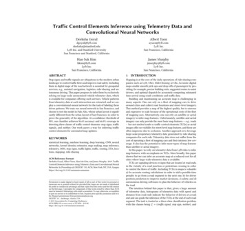
SIGKDD ’19, , Anchorage, Alaska, USAFigure 1: (Left) Histogram of vehicle speed and distancefrom the road end in North-West direction. The road endswith a stop sign, located at around 175 feet. (Right) Scatterplot of the vehicle data points used to build the histogramFigure 2: (Left) Histogram of vehicle speed and distancefrom the road end in South-West direction. The road endswith a traffic signal, located at 80 feet. (Right) Scatter plot ofthe vehicle data points used to build the histogramFigure 3: (Left) Histogram of vehicle speed and distancefrom the road end in South-West direction. The road endswith neither a stop sign, nor a traffic signal. (Right) Scatterplot of the vehicle data points used to build the histogramwe show in Fig. 1, 2 and 3, examples of such histograms for each ofthe three classes. Fig. 1 represents the histogram for a road segmentending with a stop sign, and we observe that the speed of thedrivers decreases as they approach the junction and then increasesafterwards, displaying a v shape in the histogram. Fig. 2 representsthe histogram for a road segment ending with a traffic signal, andGoyal and Yuen, et al.we see not only the similar v shape from the stop sign histogram,but also a line of constant speed, which indicates drivers goingthrough on a green light. An example of a road end with neither isshown in Fig. 3, and this idiosyncratic example reveals that manydrivers go through with constant speed. The neither class is aninteresting case because it encompasses many different types ofjunction. For the most part, however, their driver patterns differnoticeably from those of stop signs and traffic signals.We propose to use a convolutional neural network, a neuralnetwork architecture that is shift-invariant and specialized for processing data with a grid-like structure — e.g., images or histograms— to classify the three classes C. More ambitiously, by leveraginglarge-scale telemetry data, we can use this approach to successfullypredict a larger variety of map features, e.g., number of lanes orspeed bumps.This paper is organized as follows: We first provide an overviewof related work on telemetry and map inference. Geospatial applications of telemetry data range from traffic understanding down to thelevel of computing precise locations of vehicles. Map inference isthe process of inferring map features — roads, buildings, traffic control elements — mainly from telemetry data and imagery. We thendescribe the publicly available datasets as well as our anonymizedLyft proprietary dataset employed in this paper. We present themethodology of inferring TCEs from the problem formulation anddata processing to the chosen neural network architecture. We subsequently apply our trained deep learning model to San Franciscoand Palo Alto, and describe the performance of our model as wellas its limitations. Last, we suggest what can be done next to extendour present work.2RELATED WORKTelemetry data from smartphones has been used for more thana decade to develop intelligent transportation systems: to understand road usage and traffic [9, 16, 40], or to estimate arrival timefrom a place to another [20, 21]. Combined with an accurate mapof the road network, the path of a vehicle on the road networkcan be reconstructed using telemetry data, even in the case ofnoisy and sparse data [29]. Crucial for the development of intelligent transportation systems, this class of algorithms is called mapmatching [11, 19, 30]. While map-matching can be generalized forcases when the map is wrong [28], map-matching algorithms — aswell as all arrival time estimation and routing algorithms — workbest when the map is correct. Here lies the value of map inference.Most map inference work in the literature has been focused oninferring and updating the road network [1, 5, 12, 26, 33] fromGPS traces — e.g., using kernel density estimators [3, 4], iterativemethods [15], clustering algorithms [8] or graph spanners [38].With the availability of inexpensive satellite and aerial imagerydata, GPU computing power, as well as progress in convolutionalneural network (CNN) for computer vision [36, 37], CNN-poweredmap inference has been used to infer road segments at varyingdegrees of success [2, 6, 10, 17, 22, 27].Inferring traffic control elements with telemetry data has beenexplored in the past by using ruled-based methods [7, 39] in a setof manually selected candidate locations, or by using more traditional statistical learning approaches, both supervised (random
Traffic Control Elements Inference using Telemetry Data and Convolutional Neural Networksforest, Gaussian mixture models, SVM, naive Bayes) and unsupervised (spectral clustering) [18]. However, the study relied on hireddrivers who probably know the purpose of the study (which mayunconsciously bias their driving behavior) and clever but extensivefeature engineering which may not be straightforward because ofnoisy or sparse sensor data, e.g., the number of the times the vehicleis stopped and the final stop duration.This paper infers traffic control elements for map updates usingtelemetry data and a CNN-based computer vision approach. Thisdiffers from past map inference work as a) most of the past workin map inference focused on inferring the road segments for mapupdates, b) it relies too much on prior knowledge about the mapand driver behavior which means that it cannot be easily deployedin all cities, and c) the work on telemetry data was based on moretraditional statistical methods.While this present paper focuses only on the inference of trafficcontrol elements, the current approach can be generalized to manytypes of map features.3DATASETThis paper relies on three data sources:San Francisco Open Data - Our Ground Truth: Launched in2009, the City of San Francisco opened hundreds of datasets pertaining to the urbanism of San Francisco as well as its urban life.Among the available datasets are the stop signs dataset [31] — 10,527stop signs — and the traffic signal dataset [32] — 1,397 traffic signals,each of which, in that dataset, can represent multiple traffic signalsdepending on the direction of the road. While OSM also containstraffic signals and stop signs, after benchmarking the coverage andaccuracy of the OSM traffic light and stop signs datasets, we decided not to rely on the OSM traffic signal and stop signs datasetsbecause of its poor quality. The datasets from San Francisco OpenData proved to be much more reliable, and are used as ground truthto train our classifier.The Road Network in Open Street Map (OSM) - What wewant to label: OSM is an open source map whose first contributions started in 2004 [13]. We mostly rely on the road network, defined as a directed graph in which the vertices are road junctions andthe edges are roads. Our task is to label the end of each directed edgewith one of the three classes in C (traffic signal, stop sign, neither).We assume that the road network correctly models the road segments in our physical world, which is an appropriate assumptionas the road segments in the road network should first be well modeled before inferring other elements in the road network (e.g., TCE,speed limits, number of lanes, turn restrictions). In practice, an algorithm to detect road segment errors is first run. Then, the algorithmof the present paper is run.Anonymized proprietary Lyft telemetry data: We leverage Lyftvehicle telemetry data collected for forty days in the summer of2018 in San Francisco and Palo Alto, collected from smartphones.Each data point contains the latitude, longitude, accuracy, speed andbearing. A future iteration of this work could make use of morefeatures like acceleration, gyroscope, and timestamp. Contrary toRefs. [7, 18, 39], apart from building histograms, we do not engineerany additional features. Collecting driver data over a short period oftime ensures that we are capturing only the TCEs that are currentlySIGKDD ’19, , Anchorage, Alaska, USAin the road network. We want, for example, avoid the situationwhere we collect data for a long period of time (e.g., years), inferthat a given road segment possesses a TCE, but realize that the TCEwas actually removed during that period of time.We create bounding boxes over the end of each road segmentin San Francisco. We assign vehicle data points to each boundingbox, from which we extract driver patterns. 20% of bounding boxeswe looked at are reserved for testing, 20% for validation, and theremaining 60% are for training, all of which are selected randomly.We ensured that the training set and the test set are drawn fromthe same distribution.4 METHODOLOGY4.1 Problem FormulationThe TCE prediction task is a multi-label classification problem forlabeling traffic flows at junctions. The inputs are diagrams generated by applying a Kernel Density Estimator (KDE) on data points ineach bounding box (see Fig. 4), which display the frequency of datapoints found at certain speeds and distances near junctions. Notethat, for example, a four-way junction would have four diagramsfor each traffic flow into the junction. The output is a predictionfor the traffic being controlled by one of the three classes in C: astop sign, a traffic signal, or neither.We optimize for the mean cross-entropy loss function:L NN 31 ÕÕ1 ÕH (X i , yi ) yi, j log(ŷi, j ),N i 1N i 1 j 1(1)where N is the size of the dataset to compute the cross-entropyloss function, H is the cross-entropy between the output of themodel applied to the sample X i (the i-th diagrams) and the groundtruth yi , ŷi, j is the predicted probability output of the model for thesample i and the label j. yi, j 1 if j is the label for i, else yi, j 0.4.2Training Data GenerationOur pipeline for generating predictions involves three data processing steps.4.2.1 Generate Bounding Boxes. In order to know where to collectdriver telemetry data from, we create bounding boxes over the endof each road segment using the graph of the road network providedby OSM [13]. Those bounding boxes are defined by the length, thewidth, the position of the center as well as the bearing of the box.We arbitrarily decided to use a length of 57 m and a width of 47 m,and those values can be revisited in a future iteration of this work.The bearing is given by OSM. These boxes also make sure to cover10 m after the junction so that we can collect the vehicle data asvehicles enter, cross, and leave the junctions. Figures 4 and 5 showexamples of the bounding boxes.We filter out bounding boxes for junctions that have more thanfour segments as those cases are rare (around 0.01% in San Francisco). We also filter out bounding boxes for junctions that are tooclose to each other, so that we do not have any bounding boxescover more than one junction. Even after removing these cases,we retain a coverage of junctions othat is over 90% with 33,532bounding boxes as shown in Fig. 5.
SIGKDD ’19, , Anchorage, Alaska, USAWe then label the bounding boxes using the San Francisco OpenDatasets [31, 32]. They are labeled by checking which traffic controlelement in the dataset is closest to the junction in the bounding box.If there are none, then we label the bounding box as not havingany traffic control elements (neither). We have manually benchmarked this approach by randomly selecting 100 junctions fromthe San Francisco Open Datasets and validated that the 100 selectedjunctions are correct.Figure 4: Examples of bounding boxes around Baker Streetand Hayes Street in San Francisco with the following labels:Red stop sign, Yellow traffic signal, Blue neither.Goyal and Yuen, et al.4.2.2 Collect Telemetry Data. For each bounding box, we collectdriver telemetry data inside of them from 40 days in the summerof 2018 for San Francisco. These days are deliberately chosen to bedifferent days of the week to ensure that we are not overfitting fortraffic patterns on certain days. We then place each of these datapoints into the correct bounding boxes by aligning the bearing ofthe telemetry data and the bearing of the bounding box. This prevents collecting driver data in the opposite direction of traffic flow.Note that some data points may be assigned to multiple boundingboxes, since all bounding boxes at a junction cover the center partof the junction.It is likely that some data points would display low GPS accuracybecause of tall buildings in San Francisco as well as low smartphonequality. Thus, we make sure to only collect data points with highGPS accuracy.In order to have enough data points to see clear driver patterns,we only keep bounding boxes that have at least 1,000 data points.This reduces the number of bounding boxes to 24,339. For futureiterations, rather than cutting out bounding boxes with fewer datapoints, we could continue to collect telemetry in each boundingbox until we reach the lower bound.4.2.3 Kernel Density Estimators. For each bounding box, we createa diagram over speed and distance from junction by applying a 2DKernel Density Estimator (KDE) [35] on the data with a Gaussiankernel function. The bandwidth of the KDE is determined by Silverman’s rule of thumb [35].At lower speeds, we are likely to see more location data points thanat higher speeds because of the sampling rate. This leads to a noticeable amount of driver data points at speed zero at all distancesfrom the junction. These points are not indicative of any driverpattern and add noise. In order to mitigate the effect of this noise,we normalize the diagram with a cube root and min/max normalization. These normalization steps moreover help with surfacingthe driver patterns we are searching for.4.3TrainingWe use a deep learning model in order to discern the driver patterns from each diagram. We choose to train a convolutional neuralnetwork as this class of neural networks is shift-invariant and specialized for processing data with a grid-like structure, and has beenparticularly successful in solving computer vision problems [24, 25].Preprocessing of Diagrams. Before we train, we resize the diagrams to dimensions 224 x 224 x 3. We further normalize the threechannels in the images using mean [0.485, 0.456, 0.406] and std [0.229, 0.224, 0.225] in order to properly train the neural network.Figure 5: The bounding boxes in San Francisco with the labeling defined above.VGG19. Our classifier uses the VGG19 architecture [37], developed in 2014, which improves upon AlexNet [24] by developinga deeper architecture which leverages small filters. By doing so,the model is able to have the same effective receptive field as ashallower network with larger filters, but is able to have more nonlinearities and fewer parameters which increases its performance.We tried using the ResNet architecture [14] and found that therewas a negligible difference in performance. This might be becausethe input images simply contain one pattern per image, which is
Traffic Control Elements Inference using Telemetry Data and Convolutional Neural Networksmuch simpler than images that are often fed into convolutionalneural networks, making a change in architecture unnecessary.SIGKDD ’19, , Anchorage, Alaska, USAThe validation and training accuracies in Fig. 6 tend to stayaround the same, suggesting that there is little overfitting.Transfer Learning. We tried a custom neural network architecture initialized with random weights. However, we found that whenwe initialized our network with VGG19 pretrained on ImageNet,there was a significant boost in accuracy. Despite our input imagesbeing very different from the ImageNet images, transfer learninghas demonstrated the ability to detect underlying patterns effectively [34].We initialize with the weights from VGG19 pretrained on the ImageNet dataset and do not freeze any layers. We add an additionalfully connected layer to the end of the network that has randomlyinitialized weights and outputs three scores.Parameters. We decrease the learning rate by gamma after 14epochs. We also use the Adam adaptive learning update [23] withβ 1 0.9, β 2 0.999, and ϵ 1e 8. We use a batch size of 8.5 EXPERIMENTAL RESULTS5.1 Evaluation MetricsOur approach is to first get a well-trained model based on accuracyin San Francisco. We then test the model in Palo Alto to see itsgeneralizability. We evaluate this model by accuracy, precision,recall, F1 score, and coverage of dataset.Figure 7: Training: Cross-Entropy Loss over EpochLoss. The loss curves in Fig. 7 show a gradual decrease in loss.5.2Hyperparameter TuningFor hyperparameter tuning, we use the aforementioned diagramsand model architecture, and we tune the learning rate and gammadecay rate values. We find that the best learning rate and gammavalues are 0.001 and 0.1 respectively.5.3Train on San FranciscoWe trained our model using San Francisco data.Accuracy. After hyperparameter tuning, our best model for thethree classes has a validation accuracy of 91.26%.Saliency Maps. Saliency maps [36] are a useful technique forvisualizing what pixels in the input image are most essential tothe classifier in making its prediction. In the saliency maps for thismodel shown in Fig. 8, we see that the model is able to identify thedriver patterns we are searching for in each class. The stop signsaliency maps show that the model is looking for the v pattern. Thetraffic signal saliency maps show that the model is looking for anormalized v pattern since they also tend to exhibit patterns forconstant speed. Finally, the neither case shows that the model islearning multiple cases for neither junctions.5.4Test on Palo AltoIn order to evaluate how general the classifier is, we test the classifier in Palo Alto. Palo Alto is a good candidate because it is notas urban as San Francisco, so one might expect a drop in performance of the classifier. Moreover, in our dataset, San Francisco’straffic control elements comprise around 40% stop signs, 20% trafficsignals, and 40% neither. Palo Alto, on the other hand, is comprisedof around 15% stop signs, 8% traffic signals, and 77% neither. Thesepredictions are then compared against manual curation by humanexperts.Data Processing. We followed the same data processing pipelineas before to create bounding boxes around each junction in PaloAlto, collect millions of driver data points, and then assign the datapoints to each bounding box. This created 3,641 bounding boxesfor Palo Alto, which are shown in Fig. 9.Figure 6: Training: Accuracy over EpochPrediction. We apply the VGG19 classifier trained on the SanFrancisco data on the Palo Alto data to output confidence scores ineach class for each image.
SIGKDD ’19, , Anchorage, Alaska, USAGoyal and Yuen, et al.Figure 8: (Top) Examples of the input diagram for training for the three classes. (Bottom) Saliency maps for the three classesmodel assigns a confidence value greater or equal to t. By increasing the confidence threshold, we are able to increase total accuracy.However, this comes at the cost of decreasing the coverage of thedataset.If we choose a confidence threshold of t 80%, for example, themodel achieves a total accuracy of 94.874% and it covers 82.10% ofthe bounding boxes we provide.Should we want to contribute our results to the open sourcecommunity, by thresholding, we can reduce the load on manualcuration to only samples that the model is very confident in.Accuracies for each class. Table 1 shows that the classifier performs best at predicting neither junctions. This could be because theSan Francisco dataset had a large proportion of neither junctions. Infact, the model was able to predict all yield signs it encountered asneither. We are confident that with more stop sign and traffic signaltraining data, the classifier can perform better in those classes aswell.5.5Incorrect PredictionsFigure 9: The bounding boxes in Palo Alto. The orange labeling of the boxing boxes signifies that we do not currentlyknow their labels at prediction time.We look at a random sample of diagrams and their predictionsand find that the incorrect predictions can be grouped into threecategories: label limitations, outliers, and lack of data.Evaluation. A 10% quality control check on the human curatedground truth showed 97% accuracy. Compared to the ground truth,the San Francisco classifier applied to Palo Alto has a total accuracyof 90.1%. Its precision, recall, and F1 scores are 0.90.These results are promising because the model’s accuracy is similarto that in San Francisco despite Palo Alto’s traffic patterns beingwidely different.5.5.1 Label Limitations. While the San Francisco open datasetcovers many traffic control elements, there are still some limitationsto using it. For example, it does not label implied stops, such aswhen a minor street intersects with a major street. Our classifieroften predicts this as having a stop sign, since the driver at theminor street exhibits stop-sign-like behavior. This can explain whythe stop sign accuracy is lowest, while it is an effectively correctprediction.Confidence Thresholding. We can further increase the total accuracy and F1 score if we threshold by confidence as shown inTable 1. The confidence threshold t only keeps data points that the5.5.2 Outliers. As shown in Fig. 10, some junctions have outliersthat skew the histograms and thus obscure the driver patterns. Thisis resolved by filtering out extreme points.
Traffic Control Elements Inference using Telemetry Data and Convolutional Neural NetworksConfidenceThreshold 0%77.19%66.06%46.19%12.63%Palo Alto MetricsTotal Accu- Stop Sign TrafficNeither ac- 3%91.30%91.67%100%0.99Table 1: Palo Alto Confidence ThresholdingFigure 10: A few data points at high speeds are causing skew5.5.3 Insufficient Number of Data Points. Some histograms do notshow a clear pattern and these tend to have fewer data points. Wecan resolve this by raising the lower bound on number of datapoints per bounding box. This can also be corrected by the firstimprovement that we propose in the next section in order to reducethe noise level, and therefore the need to collect a larger amount ofdata point/6SIGKDD ’19, , Anchorage, Alaska, USAFUTURE WORK AND CONCLUSIONSo far, accurate and thorough data on traffic control elements hasbeen incorporated into digital maps by using street-level observations, usually from human beings or cameras. We prove in thispaper that large-scale telemetry data can be used in conjunctionwith deep learning to infer traffic control elements for automatedAverage Re- Average 00.910.950.960.970.970.99map updates, as demonstrated by the high accuracy and F1 scorein a region different from the region where the model was trained.This is a promising step forward into wide-scale traffic controlelement detection. However, we believe that further improvementscan be made.First and foremost, the most direct improvement of this work is touse map-matched drivers locations. A map-matching algorithm [28,30] takes as input the map of the road network and a sequence ofpossibly sparse and noisy locations, and outputs a trajectory on theroad network. By map-matching each ride of the drivers, we canattribute a location in the road network for each driver location(mostly collected from the GPS unit of the drivers’ smartphones).That would solve two problems: 1) Our diagram-based approachwill then successfully work in places with overlapping roads, shortroads and urban canyon, where the GPS location is notoriously lessaccurate, as we will directly collect map-matched locations data ona given road segment, and not noisy GPs locations using boundingboxes. All kind of road segments will therefore be captured. 2)Because the data collection is no longer done in a bounding boxfor each road segment, but directly on each road segment, the sizeand shape of bounding boxes being arbitrary will no longer bean issue. We would also no longer encounter the possible issue ofoverlapping bounding boxes. We would also be able to apply ourcurrent algorithm in cities with a large amount of curved roads(e.g., Paris).Another important improvement of our model would be to addmore sensory input to the model, such as acceleration. Road typeand neighborhood type should also be added as inputs to the model,as they are often correlated with the type of traffic control elements.This paper only explores three classes, but there are other typesof traffic control elements — for example, y
Han Suk Kim hkim@lyft.com Lyft Inc. San Francisco, California James Murphy jmurphy@lyft.com Lyft Inc. San Francisco, California ABSTRACT Stop signs and traffic signals are ubiquitous in the modern urban landscape to control traffic flows and improve road safety. Including them in dig