Transcription
Trajectory Tracking and Stair Climbing Capability Assessment for aSkid-Steered Mobile RobotChandrakanth R. Terupally , J.Jim ZhuΔ and Robert L. Williams II Abstract— This paper presents derivation of a trajectorytracking and stair climbing stabilization controller for a4-wheel driven skid-steered wheeled mobile robot (SSWR). Therobot vehicle is modeled with six degrees of freedom (6DOF)rigid body equations which are later simplified for planar andpitched movement. An efficient control algorithm, calledTrajectory Linearization Control (TLC), is used to tackle thechallenges posed by nonlinearities of the model. In TLC, statedynamics are linearized along the trajectory being tracked.Kinematics and dynamics of the vehicle are controlledindividually by feedback loops, where the former constitutesthe outermost loop. Simulation results promise trajectorytracking with desired accuracy. For the test prototype withcurrent physical configuration, an upper limit is found onsteepness of staircase it can safely climb. 3-sigma Monte Carloanalysis is used to show robustness of the controller toparametric perturbations.I. INTRODUCTIONSkid steered wheeled robots (SSWRs) constitute a genreof nonholonomic vehicles that lack a steering columnand are controlled by differential steer mechanism. Absenceof a steering column makes them mechanically robust andsimple to control. Compared to tracked vehicles, SSWRshave two major advantages. Firstly, an SSWR with similardimensions and weight would dissipate lesser energy inskidding turns compared to its tracked counterpart, owing tolesser area of surface contact. Secondly, SSWRs have lessertendency to slip on stair edges and sway from direction ofmaximum ascent, as wheels tend to lock up with stairs.Caracciolo et al. [1] approached planar tracking problemfor an SSWR by constraining the instantaneous centre ofrotation to between the two axles and used dynamicfeedback linearization to reduce the control problem to merekinematics. Kozilowski et al. [2] used Dixon’s [3] algorithmsbased on Lyapunov’s approach. Their technique relied onbackstepping through intensive use of coordinatetransformations making the algorithm quite complicated.Global exponential stability for transformed states wasachieved by tracking an exponentially decaying tunableoscillator signal. This methodology overcame Brockett’scondition and regulation problem was realized in contrast toCaracciolo et al. and the present paper.For stair climbing, Martens and Newman [4]experimented with an algorithm by maintaining direction ofmaximum ascent during the climb by compensating forgravity-induced drift. A proportional control law was School of EECS, Ohio University.School of EECS, Ohio University, Correspondence email: zhuj@ohio.edu. Department of Mechanical Engineering, Ohio University.Δimplemented with experimentally determined bandwidth andgain. Steplight et.al [5] developed a kinematics-based PDcontroller aided with a suite of sensors, used one at a timebased on a rule, to estimate stair profile. Xiong and Matthies[6] used robust stair edge detection techniques using a singlecamera to estimate heading angle and centre position. Theyexperimented stair climbing under various types of stairs invaried lighting conditions and shadows to prove robustnessof their algorithm. Their work was extended by Helmicket.al. [7], who used a full-fledged sensor suite withaccelerometers, vision, sonar etc. with enhanced estimationand control laws to detect and estimate stair profile. Theyclaim to have achieved climbing speeds over 1½ feet/sec.This paper aims to develop a unified controller for planartracking and autonomous stair climbing based on 6DOFdynamic model, which is briefed in section II. The 6DOFvehicle model is simplified for planar tracking andmodifications are made to the planar model to account forpitch angle during stair climbing. Section III discussesderivation of control law, followed by evaluation ofcontroller performance by means of numerical simulations.Results presented for planar tracking show desirableperformance with almost zero steady state tracking error.Robustness of the controller to parametric perturbations isinvestigated with 3-sigma Monte-Carlo simulations. Of 100simulations with randomly perturbed physical parametersand friction coefficients, 96 yielded stable results.Simulation of stair climb showed that with the currentconfiguration of the prototype robot, only a 20 staircase or a30 ramp could be safely climbed up at a speed of 0.3m/s.This unsatisfactory limit calls for design modifications to theprototype robot.Regulation problem is not addressed, as it is a concern ofthe highest level of control – the mission trajectory planner,to plan a path for the robot. Optimality decisions will bemade at the same level.II. DYNAMIC MODELINGPhysical constants are defined and their values for theprototype robot are presented below.a, distance of CG from front axle of robot 0.198 m.b, distance of CG from rear axle of robot 0.2275 m.c, half the track width 0.294 m.d, distance from instantaneous center of rotation(geometric center by choice) of robot to CG, -0.0148 m.h, height of CG above plane of surface of contact.Ixx, moment of inertia about body x-axis 11 Kgm2.Iyy moment of inertia about body y-axis 6.68 Kgm2.Izz moment of inertia about bqody z-axis 12.79 Kgm2.Ixy cross moment of inertia -0.4 Kgm2
Ixz cross moment of inertia -0.22 Kgm2.Iyz cross moment of inertia 0.9543 Kgm2.Km, motor torque constant 0.74 Nm/A.Ke, motor back-emf constant 0.8433 Vs/rad.r, radius of wheel 0.1778 m.Ra, motor armature resistance 0.22 ohms.m, mass of the robot 115.3 kg.n, motor gear ratio 1.u2 ,u3 front left and front right applied motor voltages.B. Planar MotionFor planar motion, we haveθ φ 0, ω x ω y 0, M x M y 0, v z 0, vz 01m1mFyω z vx .(6)Simplifying (1)-(4) using (5) and (6) yields a model aspresented in [1] and [2], which can be summarized as(7)p S qτ , torque produced by the motor.q M Cq M R M Bτ 1A. 6DOF Model 1 1(8)where,The following four equations summarize the 6DOF modelderived in [8].p [X Y ]TSφ Sθ Cψ Cφ SψSφ Sθ Sψ Cφ CψSφ Cθ vx Cφ Sθ Sψ Sφ Cψ v y (1) v z Cφ Cθvx 1mFx ω y v z ω z v yvy 1mFy ω z v x ω x v zvz 1mFz ω x v y ω y v x cosψ sin ψS (t ) Cφ Sθ Cψ Sφ SψDynamics of translational motion are given by(2)Kinematics of rotational motion are given byφ ω x ω y sin φ tan θ ω z cos φ tan θθ ω y cos φ ω z sin φis position vector and q [ vxω z ] isTvelocity vector;Kinematics of translational motion: X Cθ Cψ Y C S θ ψ Z Sθω y v z andFx(5)d sin ψ . d cosψ Derivation and detailed expressions for the matricesM , C , R, B are presented in [2, 9].C. Introducing Pitch into the Planar ModelPlanar dynamics presented in previous subsection aremodified to introduce static effects of stair/ramp climbing.Changes in normal reactions at wheels due to non-zero pitchare the only aspect considered. Body roll and rate of changeof pitch are neglected assuming that the vehicle is on atransversally level (unbanked) ramp/staircase and is headingin the direction of maximum ascent. A comprehensive modelof stair-climb with dynamic effects of body roll and pitch isreserved for future work.(3)ψ ω y sin φ sec θ ω z cos φ sec θDynamics of rotational motion are given byxxxxω x I xyω xω y I yzω yω z gl M x gn M zy2y2yyω y I xxω x I zzω z I xzω xω z g m M yzzzzω z I xyω xω y I yzω yω z gl M x gn M z(4)where,X , Y , Z are velocities measured in world frame; φ ,θ ,ψare Euler angles roll, pitch and yaw respectively; vx , vy ,vzare vehicle velocities measured in body frame; ω x , ω y , ω zare angular velocities of the vehicle about x,y,z axes (bodyaxes) respectively; Fx , Fy , Fz denote forces acting on centerof gravity along x,y,z axes respectively; M x , M y , M zFigure 1: Free body diagram of the vehicle on an inclined plane(Courtesy: J. Litter [10])The situation differs from planar (i.e. zero pitch) conditionin that the normal reactions are distributed unequally onwheels and, in addition, there is a component of weightpulling the robot downwards the incline.From the geometry of Figure 1 (best viewed at 250%zoom), writing torque equations about CG at surface point ofcontact of each wheel,4rio Z respectively denote total moment about body x, y and zaxes;xI xydenotes coefficient of cross moment of inertia rio N j 0, i 1, 2,3, 4(9)j 1j ioccurring in ω xω y term in the equation for ω x and gzwhere rio is the vector from the point of surface contact ofdenotes coefficient of M z in equation for ω x . Detailedi wheel to origin (CG); θ is measured positive for ascent;expressions for each of them can be found in [13].N j is the normal reaction at i wheel; Z is the resultantxthth
force vector at CG, andZ ( mv x mg sin θ cos ψ ) xˆ ( mg sin θ sin ψ ) yˆ ( mg cos θ ) zˆThe set of equations in (9) is degenerate. A particularsolution would exist if it were assumed that the vehicle isheading in the direction of maximum ascent (i.e., zero bodyroll angle). In such a case, the front wheels (and so will theback wheels) share an equal amount of reaction force.i.e., N 1 N 4 and N 2 N 3This assumption renders y component of Z to zero. Thesolution to the set of equations would now beN1 N 4 ( mgb cos θ mv x h mgh sin θ ) 2( a b )N 2 N 3 ( mga cos θ mv x h mgh sin θ ) 2( a b ) .These expressions are substituted in the planar model’sequations for frictional forces to account for non-zero pitchangle.Compared to vehicle on a ramp, stability on staircase isworsened by the bumping effect when wheels encounterstair edges, which in turn introduces random errors inheading angle leading to a natural tendency to sway awayfrom direction of steepest ascent to zero ascent. On astaircase with an inclination ‘θ’, it can be shown that thepitch angle variation due to wheel engaging the stairs is()θ, assuming that stepapproximately δθ 2 arcsin r 1 asin bheight and wheel radius are approximately equal.III. CONTROLLER DESIGNConsider the time-varying nonlinear dynamic systemξ (t ) f (ξ (t ), μ (t ), σ (t ))η (t ) h (ξ (t ), μ (t ), σ (t ))(10)where ξ (t ) is n x 1 state vector, μ (t ) is p x 1 vector of input,η (t ) is m x 1 output vector of the system, and σ(t) is a set oftime-varying parameters influencing the system behavior.Define the nominal trajectories byξ (t ) f (ξ (t ), μ (t ), σ (t ))η (t ) h(ξ (t ), μ (t ), σ (t ))(11)where an over-bar indicates nominal value of the quantity,η (t ) is the desired output being tracked, μ (t ) is the nominalPI controller using PD-eigenstructure placement techniques[11, 12, 13].Open loop control μ (t ) and nominal state ξ (t ) could becomputed with a perfect inverse system that yields identityon cascade with the actual system. In general, this is neitherpossible nor desirable. Hence, a pseudo inverse system isdesigned to estimate the nominal control input required (toachieve desired output) and PI control is used to drive thetracking errors to zero. Pseudo inverse (or equivalently,nominal control) is expected to do a fair job in keeping openloop control errors small enough so that linearization of (10)about origin (i.e. zero errors) is valid at any given point oftime.Time variable has been dropped to avoid clutter, butquantities in the above equations are not constrained to betime-invariant. Also, it is assumed that the parameter set σ(t)of the system is known and does not require to be estimatedor errors accounted for.Equation (13) when linearized, the state, input and outputwould be linear approximations of the actual errors. Hence,corresponding variables are changed while writing thelinearized tracking error dynamics as:x (t ) A (ξ (t ), μ (t ),σ ) x (t ) B (ξ (t ), μ (t ),σ ) u (t )y (t ) C (ξ (t ),μ (t ),σ ) x (t ) D (ξ (t ),μ (t ),σ ) u (t )where x (t ), u (t ), y (t ) are linearized approximations of theerror state ξ (t ) the error control input μ (t ) and the outputerror η (t ) respectively, and A, B, C, D (with dependenciesare dropped to avoid clutter) are Jacobian matrices in theTaylor expansion of (13) at [ξ , μ ] [ 0, 0 ] .Adding an integrator to the linear system in (16),x (t ) A(t ) x (t ) B (t )u (t )y (t ) C ( t ) x (t ) D ( t ) u ( t )(15)ζ (t ) x ( t )Now a state feedback PI control law is implemented asu (t ) K P (t ) x (t ) K I (t )ζ (t )(16)Substituting (16) in (15) and rewriting in matrix form,control input required, and ξ (t ) is the nominal state vector. x (t ) A(t ) B (t ) K P (t ) B (t ) K I (t ) x (t ) ζ (t ) ζ (t ) IODefine the state, input and output errors respectively asξ (t ) ξ (t ) ξ (t ), μ (t ) μ (t ) μ (t ), η (t ) η (t ) η (t ).(12) x (t ) u (t ) [ K P (t ) K I (t ) ] ζ (t ) Taking time derivative of the state error vector andeliminating ξ (t ) , μ (t ) , η (t ) , and σ (t ) using (12) yields thetracking error dynamicsξ f (ξ ξ , μ μ , σ ) f (ξ , μ , σ ) : F (ξ , μ , ξ , μ , σ )η h (ξ ξ , μ μ , σ ) h (ξ , μ , σ ) : H (ξ , μ , ξ , μ , σ )(13)The tracking error dynamics are stabilized by designing a(14)(17)Using PD-eigenstructure assignment [11, 12, 13] for thesystem in (17), for constant PD-eigenvalues, the gainsK P (t ) and K I (t ) can be evaluated for a desired polynomialλn αλ n 1 . α λ αn 110where n is the order of the system and α for i 0 to n-1iare coefficients of the polynomial.
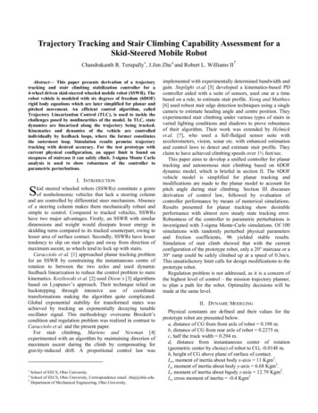
Figure 2 depicts a schematic representation of TLC.a smooth trajectory that becomes nominal input to thecontroller. The model used for simulations presented in thispaper had such a filter in inverse kinematics and inversedynamics blocks. Time varying bandwidth filter has beenfound to be advantageous over a constant bandwidth one inapplications where commands are expected to have widerange of bandwidths [11, 12, 13].IV. NUMERICAL SIMULATIONSFigure 2: Trajectory linearization control schematicA. Kinematics controllerThe procedure outlined in the preceding section is appliedto the kinematics system of (7) with p ( t ) as output. For theclosed loop system x (t ) AK (t ) BK (t ) K KP (t ) BK (t ) K KI (t ) x (t ) ,I2O2 ζ (t ) ζ (t ) (18)the expressions for PI gains KKP, KKI are evaluated usingPD-eigenvalue placement techniques. Detailed expressionscan be found in [9].Inverse KinematicsA stable and causal pseudo inversion in this case isstraightforward due to absence of zero dynamics. Inversesystem is described by the equations:q (t ) S 1( t ) p (t )(19)where p (t ) is obtained from p( t ) using a pseudodifferentiator whose bandwidth is dictated by that of theinput p ( t ) .B. Dynamics controllerThe closed loop state equation with state feedbackbecomes x ( t ) AD ( t ) BD ( t ) K DP ( t ) BD ( t ) K DI ( t ) x ( t ) . (20)I2O2 ζ ( t ) ζ ( t ) KDP, KDI are derived using PD-eigenvalue techniques.Their exact expressions (evaluated using symbolic toolboxof Matlab ) are presented in [9].Inverse DynamicsThe state (which is the output too) and input aredecoupled in forward dynamics of the robot as described by(8). It is, hence, possible to write a stable and causal pseudoinverse relation by simple rearrangement of terms as u2 1 1 q1 q1 q1 cq2 (21) u K B M q C q K 2 B q cq R 3 22121where, q is pseudo derivative of q .TLC relies on an important assumption that errors aresmall, without which linearization may be invalid. A largestep command may be sufficient to invalidate thisassumption. It is hence desired that all commands input tothe controller-plant system be smooth. This is achieved byforcing all input commands through a low pass filter called‘command shaping’ whose bandwidth depends on thetrajectories the robot is expected to track. Command shaper,typically a low pass filter, would make a step command intoPerformance of the controller is evaluated for planartracking and stair climbing by means of numericalsimulations in Matlab-Simulink. To simulate performance ofthe tracking controller, the robot is commanded to trace thecurve,32X t , Y -.002t .1t .1t , where t is time variable.Figure 3 depicts performance graphs of the controller innominal conditions. Subplot1 (1, 1) shows a bird’s eye viewof path traced by the robot, which nearly overlaps with thecommanded curve. Subplot (1,2) shows tracking error. Itfirst increases because the commanded trajectory starts witha velocity of 1.005m/s, where as the robot starts from rest.With only one integrator in the kinematics loop, this curveshould show a quadratic rise2; but as command shaping filtergains (of both outer and inner loops) are increased as timeprogresses, the deviation decreases later on. Heading angleis closely tracked and catches up almost instantaneously asshown by subplot (3,1).Initial motor voltages (subplot (2,2)) and currents (subplot(2,3)) are well within their practical limits. With Roboteqmotor controllers (AX2550) used on the test robot, 110A canbe delivered to each motor. Subplot (2,2) shows that near theend of tracking session, motor voltages approach theirsupply limit of 24v (with currently installed batteries on thetest prototype) as the robot pushes its speed beyond what itwas built for (15km/h or 4m/s).Left and right motor currents (and hence torques) as seenin subplot (2,3) change directions for the commandedtrajectory. This makes sense because the robot is initiallycommanded to turn to its left and later towards its right. Thisis exactly the same test trajectory Caracciolo et al. used in[1]. However, their torque curves didn’t show such abehavior and did not cross zero during the course, whichappears to be in error.Robustness evaluation via Monte-Carlo simulationsTo assess robustness of the controller to parametricperturbations, Monte-Carlo simulations were runprogrammatically in a loop with random dispersions inphysical parameters and friction coefficients based on anassumed normally distributed statistical model. Table 1shows various parameters with their nominal values andassumed standard deviations. Figure 4 shows performanceplots resulting from one hundred simulations for planartracking. The parameters were normally dispersed abouttheir nominal value by three times their (assumed) standard12Subplot (i,j) refers to the plot in row i and column j in the figure.The commanded curve has nonzero rate of acceleration (a jerk).
XY plot (m)Deviation From Desired Path (m)0.08300.0620TracedDesired1000100.043040XPsi Error (deg)05020-10-40010203040time (sec)Motor Currents (A)50102030time (sec)40300020000102030time (sec)4050400.08300.060010203040XPsi Error (deg)0.040.02500.5001020304050XLinear & Angular Velocities4Vx (m/s)W (rad/s)30.25201-0.25-0.50010203040time (sec)Motor Voltages (V)50100010203040time (sec)Motor Currents e (sec)40500010-201020XLinear & Angular Velocities30Vx (m/s)W (rad/s)01020time (sec)Motor Currents (A)3010050Rear Wheels0-5001020time (sec)30-1000I2I31020time (sec)30Figure 6: Performance graphs for stair climb-upDeviation From Desired Path (m)0.1YYXY plot (m)TracedDesired3010050101020time (sec)Normal Reactions (N)Front WheelsFigure 3: Nominal performance graphs20040020-40506500I2I3-2004XPsi Error (deg)-14002-20601000-2u2u300Vx (m/s)W (rad/s)Motor Voltages (V)305000.04503040XLinear & Angular Velocities20.024020142030time 0340.0220Deviation From Desired Path (m)0.04Y40XY plot (m)6Y0.1Y502030time (sec)4050Figure 4: 3-Sigma Monte-Carlo simulations simulationdeviation. Friction profiles were smoothly varied with time,within preset limits randomly unique to each simulation.TABLE ISTANDARD DEVIATIONS OF PHYSICAL PARAMETERSStandardParameterNominal ValueDeviationa0.2275 m5mmb0.1980 m5mmc0.2940 m5mmd-0.0147 m--mul0.60000.05mus0.06000.005m115.30 kg1.00 kgI12.79 kg0.50 kgr0.1778 m1mmh0.2769 m1mmKe0.84 Vs/rad0.04 Vs/radKm0.75 Nm/A0.04 Nm/ARa0.22 ohms0.02 ohmsAn exhaustive analysis of logged data and performanceplots revealed that, out of one hundred simulations, fourwent unstable (seen as spikes at end of simulation time). Inthe first instance of instability, motor torque constant Km wasperturbed by 30%, which is unrealistic for normaloperating conditions. Second instance of instability wascaused by a hike in wheel radius ‘r’ by over 6cms ( 34%).Such a variation is unusually high even if improper tireinflation is considered. In the third instance, moment ofinertia was perturbed by approximately 20%. Usingperturbation analysis, this parameter was found to be criticalfor stability at high speeds. A perturbation of 70% inarmature resistance resulted in fourth instance of instability.These cases suggest that the perturbation models need
further validation with practical situations.Stair Climbing SimulationsFigure 6 shows nominal performance simulating the robotclimbing up the stairs. Pitch angle has been chosen to be 20 plus a disturbance3 of 10 to account for bouncing effect.Simulations show that the robot tips over with any pitchangle more than this. A uniform random disturbance within 10 is added to heading (yaw angle) to account for randomerrors introduced due to slipping of tires on stair edges.Subplot (1,2) shows a maximum deviation of 40cm fromthe median of staircase during the climb. This could bedecreased by placing the controller eigenvalues farther to theleft. Performance is achieved as a trade-off with energyconsumption. Logic was implemented in the model to stopsimulation if reaction-force on front wheels becomesnegative at any point. Such situation did not arise in this 30ssimulation (at 21s, the reaction was still slightly positive).Mass and moment of inertia when individually perturbedby 1kg and 0.5kgm2 respectively, did not challenge stability.Low speed of climb (0.3m/s) also aids stability of thevehicle. Height of CG above ground critically influences thelimit of grade. An increase of 5mm in height of CG causedthe robot to tip over amid a 30sec climb up. A 20 grade istoo low for a typical indoor staircase and suggests thatimprovement is needed in mechanical design of the vehicle.V. CONCLUSIONA unified controller for planar tracking as well as stairclimbing of a SSWR has been presented. Simulation resultsshow that the TLC controller is well suited to the applicationyielding desirable results with required robustness tophysical parameters. Kozilowski et al. in [2] opined that acontrol algorithm relying on linearizing the dynamicequations is not possible due to unknown lateral skiddingforces. This paper, on contrary, shows it is indeed possible.This work will be extended to improve fidelity of thedynamic model and incorporate body roll and pitchdynamics in control design. A comprehensive evaluation ofrobustness of the controller to singular perturbations inaddition to regular perturbations should be performed.ACKNOWLEDGEMENTThis work was sponsored by Ohio University, Athens.The authors thankfully acknowledge support andsuggestions of Dr. Frank van Graas and Dr. Maarten Uijt deHaag, School of Electrical Engineering & ComputerScience, Ohio University.REFERENCES[1] Caracciolo L., De Luca A. and Iannitti S., “Trajectory trackingcontrol of a four-wheel differentially driven mobile robot”, IEEEInt. Conf. Robotics and Automation, Detroit, MI, 1999, pp. 2632–2638[2] Krzysztof Kozłowski and Dariusz Pazderski, “Modeling AndControl Of A 4-Wheel Skid-Steering Mobile Robot”, Int’l. J.Applied. Math. Computer Science, 2004, vol. 14, No. 4, pp477–496.3Disturbance was modeled as a triangular wave.[3] Dixon.W.E, Dawson.D.M., Zergeroglu.E, Behal.H, NonlinearControl of Wheeled Mobile Robots, Springer, London, 2001.[4] Martens J.D. and Newman W.S., “Stabilization of a mobile robotclimbing stairs”, Proc. IEEE International Conference on Roboticsand Automation, Page(s): 2501 -2507 vol.3, 1994.[5] Steplight.S, Egnal.G, Jung.S-H, Walker.D.B, Taylor.C.J,Ostrowski.J.P. “A Mode-Based Sensor Fusion Approach to RoboticStair-Climbing”, Proc. 2000 IEEE/RSJ International Conference onIntelligent Robots and Systems, 2000, Page(s): 1113 – 1118, vol. 2.[6] Yalin Xiong and Larry Matthies, “Vision-Guided Autonomous StairClimbing”, Proc. 2000 IEEE International Conference on Roboticsand Automation, Apr 24-28, 2000, pg.1842 -1847 vol.2.[7] Helmick D.M., Roumeliotis S.I., McHenry M.C., Matthies L.,“Multi-sensor, high speed autonomous stair climbing”, IntelligentRobots and System, 2002. IEEE/RSJ International Conference on,2002, Volume: 1, page(s): 733- 742 vol.1[8] Robert Nelson, Flight Stability and Automatic Control, 2nd edition,McGraw Hill[9] Chandrakanth Terupally, “Trajectory tracking control and stairclimbing stabilization of a skid–steered mobile robot”, masters’thesis, Dept of Electrical Engineering and Computer Science, OhioUniversity, Athens, Nov 2006.[10] J.Litter, “Mobile robot for search and rescue”, masters’ thesis, Dept.Mechanical Eng. Ohio University, Athens, June 2004.[11] C. M. Mickle, “Nonlinear Tracking Control Using A RobustDifferential-Algebraic Approach”, Ph. D. Dissertation, Dept. ofElectrical and Computer Engineering, Louisiana State University,Baton Rouge, Louisiana, Dec. 1998.[12] M.C. Mickle, Rui Huang, J. Zhu, “Unstable, Non-minimum ntrol,” Proceedings, 2004 IEEE Conference on ControlApplications, pp. 812-818, Taipei, Taiwan, Sept. 2004.[13] R. Huang, M. C. Mickle, and J. Zhu, “Nonlinear Time-varyingObserver Design Using Trajectory Linearization,” Proceedings,2003 American Control Conference, pp. 4772-4778, Denver, CO,June, 2003.
experimented stair climbing under various types of stairs in varied lighting conditions and shadows to prove robustness of their algorithm. Their work was extended by Helmick et.al. [7], who used a full-fledged sensor suite with accelerometers, vision, sonar etc. with enhanced estimation and control laws to