Transcription
FEATURE LEARNING WITH DEEP SCATTERING FOR URBAN SOUND ANALYSISJustin Salamon1,2 and Juan Pablo Bello21Center for Urban Science and Progress, New York University, USAMusic and Audio Research Laboratory, New York University, USA{justin.salamon, jpbello}@nyu.edu2ABSTRACTIn this paper we evaluate the scattering transform as an alternative signal representation to the mel-spectrogram in thecontext of unsupervised feature learning for urban sound classification. We show that we can obtain comparable (or better)performance using the scattering transform whilst reducingboth the amount of training data required for feature learningand the size of the learned codebook by an order of magnitude. In both cases the improvement is attributed to the local phase invariance of the representation. We also observeimproved classification of sources in the background of theauditory scene, a result that provides further support for theimportance of temporal modulation in sound segregation.Index Terms— Unsupervised learning, scattering transform, acoustic event classification, urban, machine learning1. INTRODUCTIONAudio classification systems have traditionally relied on handcrafted features, a popular choice being the Mel-FrequencyCepstral Coefficients (MFCCs) [1]. Examples of systems thatrely on manually engineered features in the domain of environmental sound source classification include [2–4]. Recent studies in audio classification have shown that accuracycan be improved by using unsupervised feature learning techniques as an alternative to manually designed features, withexamples in the areas of bioacoustics [5], music informationretrieval [6–8] and environmental sound classification [9–11].Still, the raw audio signal is not suitable as direct input toa classifier due to its extremely high dimensionality and thefact that it would be unlikely for perceptually similar soundsto be neighbours in vector space [5]. As a consequence,even systems that use feature learning need to first transformthe signal into a representation that lends itself to successfullearning. For audio signals, a popular representation is themel-spectrogram [5, 6, 11].In [11], we studied the application of unsupervised feature learning from mel-spectrograms for urban sound sourceThis work was supported by a seed grant from New York University’sCenter for Urban Science and Progress (CUSP).classification. We showed that the learned features can outperform MFCCs due to their ability to capture the short-termtemporal dynamics of the sound sources – a particularly important trait when dealing with sounds such as idling enginesor jackhammers whose instantaneous noise-like characteristics can be hard to distinguish otherwise. To achieve thelearning of temporal dynamics we applied frame shingling,i.e. the features were learned from groups of several consecutive frames (2D time-frequency patches). Whilst we wereable to improve classification accuracy in this way, we notedthat the downside to the approach was that we had to learna separate codeword (feature) to encode every phase-shiftwithin a 2D patch, which consequently required learning alarger codebook (set of features) overall.Over the years we have seen the advent of alternative signal representations (i.e. transforms) for audio classification,and in particular representations that encode amplitude modulation over time such as the modulation spectrogram [12,13]and more recently the scattering transform [14–16]. The latterin particular, also referred to as the deep scattering spectrum,has been shown to be stable to time-warping deformationsand capable of characterizing time-varying structure over (relatively) long window sizes compared to those used for computing MFCCs for instance. This suggests that the scatteringtransform could characterize the short-term temporal dynamics captured by 2D mel-spectrogram patches with the addedadvantage of being phase invariant. From the sound perception and cognition literature we know that modulation playsan important role in sound segregation and the formation ofauditory images [17–19], which further motivates the exploration of representations such as the scattering transform formachine listening. It has already been shown to be a usefulrepresentation for environmental sound classification in [20],although no feature learning was applied in that study.In this paper we study the use of the scattering transformin combination with the feature learning and classificationpipeline proposed in [11] for the classification of urban soundsources. In Section 2 we describe the signal representationscompared in this study. The feature learning and classificationalgorithms we use are described in Section 3, and our datasetand experimental design in Section 4. Results are discussedin Section 5 and a summary is provided in Section 6.
2. SIGNAL REPRESENTATIONS2.1. Mel SpectrogramThe mel-spectrogram is obtained by taking the short-timeFourier transform and mapping its spectral magnitudes ontothe perceptually motivated mel-scale [21] using a filterbankin the frequency domain. It is the starting point for computing MFCCs [1], and a popular representation for many audioanalysis algorithms including ones based on unsupervisedfeature learning [5–7, 11]. As in [11], we compute log-scaledmel-spectrograms with 40 bands between 0-22050 Hz using a23 ms long Hann window (1024 samples at a sampling rate of44.1 kHz) and a hop size of equal length. The representationis computed using the Essentia library [22] which providesPython bindings to a C implementation.In a feature learning framework (cf. Section 3), we canchoose to learn features from individual frames of the melspectrogram or alternatively group the frames into 2D patches(by concatenating them into a single longer vector) and applythe learning algorithm to the patches. In [11] we showed thatthe latter approach facilitates the learning of features that capture short-term temporal dynamics, outperforming MFCCsfor classification. Following this result, we group consecutiveframes to form 2D patches with a time duration of roughly370 ms. Given our analysis parameters this corresponds togrouping every 16 consecutive frames.2.2. Scattering TransformAs noted in the introduction, grouping mel-spectrogramframes captures temporal structure at the cost of having tolearn a larger number of features to cover all possible phaseshifts of a sound pattern within a 2D patch. An alternativesolution would be to use a transform that can characterize amplitude modulations in a phase-invariant way: the scatteringtransform [16].The scattering transform can be viewed as an extensionof the mel-spectrogram that computes modulation spectrumcoefficients of multiple orders through cascades of waveletconvolutions and modulus operators. Given a signal x, thefirst order (or “layer”) scattering coefficients are computed byconvolving x with a wavelet filterbank ψλ1 , taking the modulus, and averaging the result in time by convolving it with alow-pass filter φ(t) of size T :S1 x(t, λ1 ) x ψλ1 φ(t).(1)The wavelet filterbank ψλ1 has an octave frequency resolution Q1 . By setting Q1 8 the filterbank has the same frequency resolution as the mel filterbank, and this layer is approximately equivalent to the mel-spectrogram. The secondorder coefficients capture the high-frequency amplitude modulations occurring at each frequency band of the first layerand are obtained by:S2 x(t, λ1 , λ2 ) x ψλ1 ψλ2 φ(t).(2)The octave resolution of the second order filterbank is determined by Q2 . Following [16] we set Q2 1. Higher ordercoefficients can be obtained by iterating over this process, butit has been shown that for the value of T used in this study (seebelow) most of the signal energy is captured by the first andsecond order coefficients [16]. Furthermore, adding higherorder coefficients would blow-up the dimensionality of therepresentation. Consequently, in this study we use the firstand second orders for our scattering representation.It is beyond the scope of this paper to describe the scattering transform in greater detail, and we refer the interestedreader to [14–16] for further information. It will suffice tonote that the important parameters of the transform relevant toour experiments are the filterbank resolutions Q1 and Q2 andthe duration T of the averaging filter which also representsthe duration of the modulation structure we hope to captureusing the second order coefficients. As noted above, we fixQ1 8 and Q2 1. The filterbank is constructed of 1D Morlet wavelets. We set T to the same duration covered by the 2Dmel-spectrogram patches, i.e. 370 ms (for a sampling rate of44.1 kHz this implies T 1024 16). To compute the scattering transform we use the ScatNet v0.2 Matlab software1 .By default ScatNet computes the scattering coefficients without any oversampling, meaning the time-difference betweenconsecutive frames is T /2. ScatNet provides an oversamplingparameter that allows us to obtain a finer temporal representation of the transform. By modifying this parameter we canemulate different hop sizes ranging from T /2 down to thehop size we use for the mel-spectrograms (T /16). Importantly, note that the hop size is in inverse relationship to thenumber of analysis frames and consequently to the amount ofdata used for unsupervised feature learning. For each framewe concatenate the first order coefficients with all of the second order coefficients into a single feature vector. The secondorder coefficients are normalized using the previous order coefficients as described in [16]. Note that we also experimentedwith using the second order coefficients only, but this optionresulted in significantly lower classification accuracies and ishence not explored further in this study.3. FEATURE LEARNING & CLASSIFICATION3.1. Feature learning with spherical k-meansGiven our representation (log-mel-spectrogram patches orscattering transform frames), we learn a codebook of representative codewords from the training data. The samples inthe dataset are then encoded against this codebook and theresulting code vectors are used as feature vectors for training/ testing a classifier. To learn the codebook we use the spherical k-means algorithm [23]. Unlike the traditional k-meansclustering algorithm [24], the centroids are constrained tohave unit L2 norm (they must lie on the unit sphere), the1 http://www.di.ens.fr/data/software/scatnet/
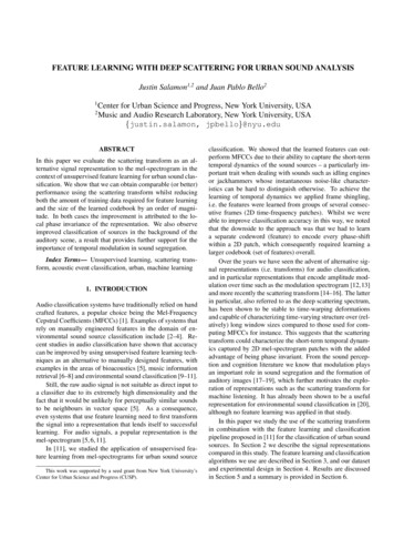
benefits of which are discussed in [23, 25]. The algorithmhas been shown to be competitive with more complex (yetconsiderably slower) techniques such as sparse coding, andhas been used successfully to learn features from audio formusic [6], birdsong [5] and urban sound classification [11].As a feature learning technique, we use the algorithm to learnan over-complete codebook, so k is typically much largerthan the dimensionality of the input data. For further detailsabout the algorithm the reader is referred to [23].Before passing the log-mel-spectrogram patches or scattering transform frames to the clustering algorithm we first reduce the dimensionality of the input data by decorrelating theinput dimensions using PCA whitening. This has been shownto significantly improve the discriminant power of the learnedfeatures [23]. Following the procedure proposed in [6], weapply PCA whitening and keep enough components to explain 99% of the variance. Empirically, this reduces the dimensionality of a mel-spectrogram patch from 640 to 250,and of a scattering frame from 427 to 230. The clusteringproduces a codebook matrix with k columns, where each column represents a codeword. Every sample in our dataset isencoded against the codebook by taking the scalar productbetween each of its frames (or patches) and the codebook matrix. This approach was shown to work better than e.g. vectorquantization [8] for the dataset studied in this paper [11]. Finally, we have to summarize the per-frame (or per-patch) values produced by the encoding over the time axis to ensure thatall samples in the dataset are represented by a feature vectorof the same dimensionality. Following [11] we summarizethe encoded values over time with two statistics: the meanand standard deviation. The resulting feature vectors are thusall of size 2k, and we standardize them across samples beforepassing them on to the classifier.3.2. ClassificationFor each representation we experimented with two differentclassification algorithms: a random forest classifier [26] with500 trees and a support vector machine [27] with a radial basis function kernel. In this way we can select the classifierthat is best suited for each representation and focus on comparing the best results obtained by the two representations.Based on these experiments, we use the random forest classifier for the mel-spectrograms and the support vector machine for the scattering transform. For both classifiers weuse the implementation provided in the scikit-learn Pythonlibrary [28] with their default hyper-parameter values.4. EXPERIMENTAL DESIGNWe use the UrbanSound8K [29] dataset for our experiments.It contains 8732 audio samples of up to 4 seconds in durationtaken from real field recordings. The samples include soundsfrom 10 classes: air conditioner, car horn, children playing,dog bark, drilling, engine idling, gun shot, jackhammer, sirenand street music; and come divided into 10 stratified subsetsfor unbiased cross-validation. Since the samples come fromfield recordings, there are often other sources present in addition to the labeled source. For each sample the dataset indicates whether the labeled source is in the foreground or background (as subjectively perceived by the dataset annotators).Each experiment is run using 10-fold cross validationbased on the stratified subsets. We compute the classificationaccuracy for each fold and present the results as a box plot.5. EXPERIMENTS & RESULTS5.1. Experiment 1: Mel-spectrogram versus ScatteringIn our first experiment, we compare the classification accuracy obtained when using the mel-spectrogram as input versus the scattering transform, varying the size k of the codebook from 200 to 2000. For this experiment we over-samplethe scattering transform such that it contains the same number of analysis frames as the mel-spectrogram. In this wayboth representations produce the same amount of training data(frames) for the feature learning algorithm.The results are presented in Figure 1. As reference, notethat a baseline system using MFCCs with a random forest(and no learning) obtained a mean accuracy of 0.69 for thesame dataset [11]. The first thing we see is that the scatteringtransform produces comparable results to the shingled melspectrogram (it actually outperforms the mel-spectrogram inthe best case, but the difference is not statistically significant).Both outperform the MFCC baseline (statistically significantaccording to a paired t-test with p 0.05). Whilst we had togroup frames into 2D patches to capture the temporal structure of sounds with mel-spectrograms, we see that this information is captured by a single frame of the scattering transform (with first and second order coefficients), as one mightexpect. The more remarkable result is that whilst the performance using the mel-spectrogram increases as we increase k,using the scattering transform we actually get better performance with smaller values of k (the best being k 500).This can be explained by the local phase invariance of thelatter: when using mel-spectrogram patches we need to learnfeatures to encode every phase-shift of a sound within a patch,whereas a scattering transform frame is invariant to this shift.This means we can obtain the same classification accuracywhilst reducing the size of the codebook by an order of magnitude. This could have a significant influence on the computational cost of the approach as we scale the problem to largerdatasets with more classes and more training samples. Notethat in practice computing the scattering transform will takelonger than computing the mel-spectrogram by a multiplicative factor proportionate to the dimensionality of the scattering output, so the effective gain in efficiency will depend onthe specific parameterization used.
0.80k 500k 1000k 2000Accuracyk 2000.750.700.650.60Fig. 1. Classification accuracy results: mel-spectrogram withfeature learning vs. scattering transform with feature learning.The codebook size k is varied from 200 to 2000.1.2M600K300K150KFig. 2. Classification accuracy for the scattering transform(with k 500) as a function of the training data size.All samplesForeground5.2. Experiment 2: Scattering OversamplingBackgroundIn our first experiment we oversampled the scattering transform so that the number of analysis frames equaled the number of frames in the mel-spectrogram. In our second experiment, we compute the scattering transform with different degrees of oversampling: from 43 frames per second (equivalent to the analysis hop size of the mel-spectrogram of 23ms) down to the critical sampling rate of the transform coefficients of 5.5 frames per second (a hop size of 185 ms). This inturn affects the total number of training frames produced forthe feature learning stage: from approximately 1.2M down to150K. Based on the results of the previous experiment, we fixk 500.In Figure 2 we present the classification accuracy obtainedas a function of the size of the data used for unsupervised feature learning. The results are somewhat surprising – ratherthan observing a decrease in performance as we decrease thesize of data, the results remain stable. As with the previous experiment, this is likely due to the local phase invariance of the scattering transform: there is no need to representevery phase shift of a 2D patch in the training data since asingle scattering frame represents all possible shifts simultaneously. Together with the findings of the previous experiment, the results are highly encouraging – by replacing themel-spectrogram with the scattering transform we are able toreduce both the amount of training data and the size of thelearned codebook by an order of magnitude whilst maintaining (or even improving) the classification accuracy.5.3. Experiment 3: Foreground versus BackgroundFinally, recall that each sample in the dataset is also labeledas being in the foreground or background. In Figure 3 weplot the best classification accuracy for the mel-spectrogramand the scattering transform alongside a breakdown into foreground accuracy and background accuracy. Whilst for theforeground sounds the representations produce very similarresults (mean accuracies of 0.814 and 0.817 respectively), weobserve a considerable improvement for background soundsFig. 3. Best classification accuracy obtained using the mel-spectrum and scattering transform with a breakdown intoforeground and background.using the scattering transform: 0.557 vs. 0.604. Though further investigation would be required to make any hard claims,our results align nicely with those of the sound perception andcognition literature [17–19], suggesting that the scatteringtransform representation better facilitates the (machine) segregation of sound sources due to its characterisation of modulation, in particular when the source of interest is masked byother sounds.6. SUMMARYIn this paper we evaluated the use of the scattering transformas an alternative to the mel-spectrogram in the context of unsupervised feature learning for environmental sound classification. We showed that we can obtain comparable (or slightlybetter) performance using the scattering transform whilst reducing both the amount of training data required for featurelearning and the size of the learned codebook by an order ofmagnitude. In both cases the improvement is attributed to thelocal phase invariance of the representation. We also notedthat the observed increase in performance was primarily dueto the improved classification of sources in the backgroundof the auditory scene, a result which aligns with the evidencefound in the sound perception and cognition literature aboutthe importance of temporal modulation for sound segregation.
REFERENCES[1] T. Ganchev, N. Fakotakis, and G. Kokkinakis, “Comparative evaluation of various MFCC implementationson the speaker verification task,” in 10th Int. Conf. onSpeech and Computer, Greece, Oct. 2005, pp. 191–194.[2] R. Radhakrishnan, A. Divakaran, and P. Smaragdis,“Audio analysis for surveillance applications,” in IEEEWASPAA’05, 2005, pp. 158–161.[3] L.-H. Cai, L. Lu, A. Hanjalic, H.-J. Zhang, and L.-HCai, “A flexible framework for key audio effects detection and auditory context inference,” IEEE TASLP, vol.14, no. 3, pp. 1026–1039, 2006.[4] T. Heittola, A. Mesaros, A. Eronen, and T. Virtanen,“Context-dependent sound event detection,” EURASIPJASMP, vol. 2013, no. 1, 2013.[5] D. Stowell and M. D. Plumbley, “Automatic large-scaleclassification of bird sounds is strongly improved by unsupervised feature learning,” PeerJ, vol. 2, pp. e488,Jul. 2014.[6] S. Dieleman and B. Schrauwen,“Multiscale approaches to music audio feature learning,” in 14th ISMIR, Curitiba, Brazil, Nov. 2013.[7] P. Hamel, S. Lemieux, Y. Bengio, and D. Eck, “Temporal pooling and multiscale learning for automatic annotation and ranking of music audio.,” in 12th ISMIR,Oct. 2011, pp. 729–734.[8] Y. Vaizman, B. McFee, and G. Lanckriet, “Codebookbased audio feature representation for music information retrieval,” IEEE TASLP, vol. 22, no. 10, pp. 1483–1493, Oct. 2014.[9] S. Chaudhuri and B. Raj, “Unsupervised hierarchicalstructure induction for deeper semantic analysis of audio,” in IEEE ICASSP, 2013, pp. 833–837.[10] E. Amid, A. Mesaros, K. J Palomaki, J. Laaksonen, andM. Kurimo, “Unsupervised feature extraction for multimedia event detection and ranking using audio content,”in IEEE ICASSP, Italy, May 2014, pp. 5939–5943.[11] J. Salamon and J. P. Bello, “Unsupervised feature learning for urban sound classification,” in IEEE ICASSP,Brisbane, Australia, Apr. 2015.[12] L. Atlas and Shihab A. Shamma, “Joint acoustic andmodulation frequency,” EURASIP J. on Applied SignalProcessing, vol. 2003, pp. 668–675, Jan. 2003.[13] N. H. Sephus, A. D. Lanterman, and D. V. Anderson,“Modulation spectral features: In pursuit of invariantrepresentations of music with application to unsupervised source identification,” J. of New Music Research,vol. 44, no. 1, pp. 58–70, 2015.[14] J. Andén and S. Mallat, “Multiscale scattering for audio classification,” in 12th Int. Soc. for Music Info. Re-trieval Conf., Miami, USA, Oct. 2011, pp. 657–662.[15] J. Andén and S. Mallat, “Scattering representation ofmodulated sounds,” in 15th DAFx, UK, Sep. 2012.[16] J. Andén and S. Mallat, “Deep scattering spectrum,”IEEE Trans. on Signal Processing, vol. 62, no. 16, pp.4114–4128, Aug. 2014.[17] S. McAdams, Spectral fusion, spectral parsing and theformation of auditory images, Ph.D. thesis, StanfordUniversity, Stanford, USA, 1984.[18] W.A. Yost, “Auditory image perception and analysis:The basis for hearing,” Hearing Research, vol. 56, no.1, pp. 8–18, 1991.[19] R.P. Carlyon, “How the brain separates sounds,” Trendsin cognitive sciences, vol. 8, no. 10, pp. 465–471, 2004.[20] C. Bauge, M. Lagrange, J. Anden, and S. Mallat,“Representing environmental sounds using the separable scattering transform,” in IEEE ICASSP, Vancouver,Canada, May 2013, pp. 8667–8671.[21] S. S. Stevens, J. Volkmann, and E. B. Newman, “Ascale for the measurement of the psychological magnitude pitch,” JASA, vol. 8, no. 3, pp. 185–190, 1937.[22] D. Bogdanov, N. Wack, E. Gómez, S. Gulati, P. Herrera, O. Mayor, G. Roma, J. Salamon, J. Zapata, andX. Serra, “ESSENTIA: an audio analysis library formusic information retrieval,” in 14th Int. Soc. for MusicInfo. Retrieval Conf., Brazil, Nov. 2013, pp. 493–498.[23] A. Coates and A. Y. Ng, “Learning feature representations with K-means,” in Neural Networks: Tricks of theTrade, pp. 561–580. Springer, 2012.[24] S. Lloyd, “Least squares quantization in PCM,” IEEETrans. on Information Theory, vol. 28, no. 2, pp. 129–137, 1982.[25] I.S. Dhillon and D.M. Modha, “Concept decompositions for large sparse text data using clustering,” Machine Learning, vol. 42, no. 1, pp. 143–175, 2001.[26] L. Breiman, “Random forests,” Machine Learning, vol.45, no. 1, pp. 5–32, 2001.[27] C. Cortes and V. Vapnik, “Support-vector networks,”Machine Learning, vol. 20, no. 3, pp. 273–297, 1995.[28] F. Pedregosa, G. Varoquaux, A. Gramfort, V. Michel,B. Thirion, O. Grisel, M. Blondel, P. Prettenhofer,R. Weiss, V. Dubourg, J. Vanderplas, A. Passos,D. Cournapeau, M. Brucher, M. Perrot, and E. Duchesnay, “Scikit-learn: Machine learning in python,” J.Mach. Learn. Res., vol. 12, pp. 2825–2830, 2011.[29] J. Salamon, C. Jacoby, and J. P. Bello, “A dataset andtaxonomy for urban sound research,” in 22nd ACM International Conference on Multimedia (ACM-MM’14),Orlando, FL, USA, Nov. 2014.
FEATURE LEARNING WITH DEEP SCATTERING FOR URBANSOUNDANALYSIS Justin Salamon1,2 and Juan Pablo Bello2 1Center for Urban Science and Progress, New York University, USA 2Music and Audio Research Laboratory, New York University, USA fjustin.salamon, jpbellog@nyu.edu ABSTRACT In this paper we evaluate the scattering transform as an al-