Transcription
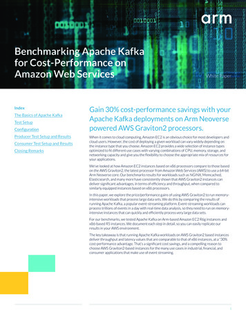
Benchmarking Apache Kafkafor Cost-Performance onAmazon Web ServicesIndexThe Basics of Apache KafkaTest SetupConfigurationProducer Test Setup and ResultsConsumer Test Setup and ResultsClosing RemarksWhite PaperGain 30% cost-performance savings with yourApache Kafka deployments on Arm Neoversepowered AWS Graviton2 processors.When it comes to cloud computing, Amazon EC2 is an obvious choice for most developers andcloud users. However, the cost of deploying a given workload can vary widely depending onthe instance type that you choose. Amazon EC2 provides a wide selection of instance typesoptimized to fit different use cases with varying combinations of CPU, memory, storage, andnetworking capacity and give you the flexibility to choose the appropriate mix of resources foryour applications.We’ve looked at how Amazon EC2 instances based on x86 processors compare to those basedon the AWS Graviton2, the latest processor from Amazon Web Services (AWS) to use a 64-bitArm Neoverse core. Our benchmarks results for workloads such as NGINX, Memcached,Elasticsearch, and many more have consistently shown that AWS Graviton2 instances candeliver significant advantages, in terms of efficiency and throughput, when compared tosimilarly equipped instances based on x86 processors.In this paper, we explore the price/performance gains of using AWS Graviton2 to run memoryintensive workloads that process large data sets. We do this by comparing the results ofrunning Apache Kafka, a popular event-streaming platform. Event-streaming workloads canprocess trillions of events in a day with real-time data analysis, so they need to run on memoryintensive instances that can quickly and efficiently process very large data sets.For our benchmarks, we tested Apache Kafka on Arm-based Amazon EC2 R6g instances andx86-based R5 instances. We document each step in detail, so you can easily replicate ourresults in your AWS environment.The key takeaway is that running Apache Kafka workloads on AWS Graviton2 based instancesdeliver throughput and latency values that are comparable to that of x86 instances, at a “30%cost-performance advantage. That’s a significant cost savings, and a compelling reason tochoose AWS Graviton2-based instances for the many use cases in industrial, financial, andconsumer applications that make use of event streaming.1
The Basics of Apache KafkaApache Kafka is an open-source platform for event streaming, designed to manage real-timedata feeds. Kafka makes it possible to analyze data that pertains to a particular event – such aswhen a sensor transmits data, a company deposits money in a bank account, or a person books ahotel room – and then respond to that event in real time.Kafka workloads can read (subscribe to) and write (publish) real-time events that occur withinan application or service and then store them for immediate use or later retrieval. Kafkaworkloads can also manipulate, process, and react to event streams, either in real time orretrospectively, and can route streams to different destination technologies as needed.Kafka workloads are used in a wide range of applications that deal with massive amounts of dataand require real-time decision-making. In the financial sector, for example, Kafka workloads canbe used to process payments, purchase stocks, and complete other transactions in real time,and in the supply chain they can be used for real-time fleet management, shipment tracking,and other logistical tasks. Industrial applications can use Kafka to capture and analyze sensordata from IoT devices and other equipment, and hospitals can use them to monitor patients andensure timely treatment. Consumer interactions become more responsive with Kafka becausehotel bookings, airline purchases, and other retail activities become both more individual andmore automatic. Enterprises can use Kafka workloads, too, using them to connect, store, andmake data more readily available throughout the organization, and as the foundation for dataplatforms, event-driven architectures, and microservices.Test SetupOur benchmark measures the throughput and latency of writing and reading events on a Kafkacluster. The throughput metric we use is Records Per Second (RPS), and the latency metric isthe 99-percentile latency in milliseconds (ms).In Kafka, events are ca lled records. Records are written by producers and read by consumers.We wanted to get a sense for the factors that influence producer and consumer performance,so we designed our tests to stress the Kafka cluster as much as possible.Keep in mind that we used a synthetic testing environment, so results on other use cases mayvary from what is shown below.2.1 Top-Level Test SetupBelow is the AWS setup for our tests.AWS Test Setup forKafka BenchmarkAWS CloudRegion us-east-1VPCZookeeper ClusterM6gM6gM6g3x M6g.xlargeLoad GeneratorsProducers/ConsumersM6gKafka Cluster (System Under Test)M6gM6gM6gM6g3-Node Kafka Cluster2X M6g.16xlarge2
The setup includes three components: a Zookeeper cluster, a Kafka cluster, and load generators.1: Zookeeper clusterThe three-node Zookeeper cluster is required for Kafka operation, and because it is not in theperformance critical path, it remained unchanged throughout all tests. To show that Zookeeperworks on Arm-based platforms without modification, we ran the cluster on general-purposem6g.xlarge instances based on the AWS Graviton2 processor.2: Kafka clusterThe three-node Kafka cluster is responsible for storing and serving records, as well as recordreplication (durability). This is the portion of the setup we stress tested. The diagram shows thatthe Kafka cluster is composed of m6g instances. However, as part of our testing we also testedthree-node clusters with the instance types and sizes shown in Table 1. Note that the instancetype with the lowest cost (USD/hr) is the AWS Graviton2 r6g.xlarge.Instance TypeSizeVirtual CPUs(vCPUs)RAM (GiB)Network (Gbps)Cost(USD/hr)Elastic Block Store(EBS) Volume (GiB)Direct Attached r6gd2xlarge432100.252None1 x 475r6gd2xlarge864100.576None1 x 300Load generatorsTable 1. Instances Usedfor Kafka Cluster 3.We ran the producer and consumer tests on the two load generator instances in the diagram.When evaluating throughput, we used both load generators, but when evaluating latency, weused only one.The table below lists key SW versions used for testing.Table 2. VersionInformationUbuntu20.04Arm AMIami-008680ee60f23c94bX86-64 AMIami-0758470213bdd23b1KafkaKafka 2.6.0 (built with Scala 2.13)ZookeeperPackaged with Kafka 2.6.0JDKopenjdk-14-jdk (installed via apt)3
Configuration3.1 Linux ConfigurationExcept for some network settings, we left the kernel-level configurations at their defaults.Below are the commands used to change the networking settings.########## To view the default value before writing, remove theassignment.# For example, to view net.ipv4.ip, run “sysctl net.ipv4.iplocal port range”sysctl net.ipv4.ip local port range ”1024 65535”sysctl net.ipv4.tcp max syn backlog 65535sysctl net.core.rmem max 8388607sysctl net.core.wmem max 8388607sysctl net.ipv4.tcp rmem ”4096 8388607 8388607”sysctl net.ipv4.tcp wmem ”4096 8388607 8388607”sysctl net.core.somaxconn 65535sysctl net.ipv4.tcp autocorking 0#########3.2 Kafka Node StorageFor instances without direct-attached storage (r6g, r5, r5a), we used Elastic Block Storage (EBS)volumes of size 512GiB. These volumes were dedicated to Kafka to ensure high performance.For instances with direct-attached storage (r6gd, r5d), we used the direct-attached storageprovided by the instance. This storage was also dedicated to Kafka to ensure high performance.Note: EBS volumes larger than 170GiB are granted more bandwidth by AWS. This is explainedin the AWS user guide for EBS volume types.3.3 Zookeeper Cluster ConfigurationBelow is the Zookeeper config file used on the three Zookeeper nodes.#############tickTime 2000dataDir /tmp/zookeeperclientPort 2181maxClientCnxns 0initLimit 10syncLimit 5server.1 zk 1 ip:2888:3888server.2 zk 2 ip:2888:3888server.3 zk 3 ip:2888:3888#############4
3.4 Kafka Cluster ConfigurationBelow is the Kafka config file used on the three Kafka nodes.############## Config parameters are documented at ion############################# Base Settings#############################broker.id unique idzookeeper.connect zk 1 ip:2181,zk 2 ip:2181,zk 3 ip:2181zookeeper.connection.timeout.ms 60000############################# Log Basics#############################log.dirs /data/kafka-logs############################# Socket Settings#############################listeners PLAINTEXT://:9092num.network.threads 24num.io.threads 32socket.send.buffer.bytes -1socket.receive.buffer.bytes -1############################# Group Coordinator .rebalance.delay.ms 0#############3.5 Topic ConfigurationKafka requires records to be stored in topics. We created separate topics for the producer andconsumer tests. We also deleted the topic after each test run.Below is the creation command for the producer test topic.#######./kafka 2.13-2.6.0/bin/kafka-topics.sh --create --topicproducer-load-test --bootstrap-server node 1 ip:9092,node 2ip:9092,node 3 ip:9092 --replication-factor 3 --partitions 64#######And here is the creation command for the consumer test topic.########./kafka 2.13-2.6.0/bin/kafka-topics.sh --create --topicconsumer-load-test --bootstrap-server node 1 ip:9092,node 2ip:9092,node 3 ip:9092 --replication-factor 3 --partitions 64########5
A few notes about the command switches used in the test topic commands:--topicThis is the name of the topic we are creating.--replication-factorSet to three since we have three nodes in the cluster. Each node will contain a copy of eachrecord committed into the cluster. Selecting a replication factor of three increases the stress onthe cluster because the follower nodes are required to act as internal consumers to replicaterecords.--partitionsSet to 64 because we found that this yields the highest throughput.Producer Test Setup and Results4.1 Producer Test Command and ConfigurationWe used the performance tests that come packaged with Kafka releases. The producerperformance test is in the Kafka bin directory, under the name kafka-producer-perf-test.sh.Below is a sample command line for the producer test.#########./kafka 2.13-2.6.0/bin/kafka-producer-perf-test.sh --printmetrics --topic producer-load-test --num-records num records--throughput -1 --record-size 100 --producer-props bootstrap.servers node 1 ip:9092,node 2 ip:9092,node 3 ip:9092 acks 1buffer.memory 67108864 batch.size 65536 linger.ms 3#########Four instances of the above command were run simultaneously. Since we had two loadgenerators, we ran two instances of this test on each load generator. We found this maximizedload on the Kafka cluster. To determine throughput (RPS), we aggregated the reportedthroughput of each of the producer instances.To determine latency, it does not make sense to aggregate latency percentiles, so we ran a singleproducer with a single instance of the above command. As a result, our latency test resultsshould be taken as a best case.A few comments about the switches in the sample command:--topicSelects the topic we write our records into.--num-recordsThe number of records to write is shown as a variable because we tested with varying recordcounts.--throughputSet to -1, which means the test executed with no limiting on the request rate. In our testing, wefound that not using rate-limiting resulted in the highest bandwidth (i.e., highest RPS).--record-sizeWe used 100-byte records for all tests. We selected a small record size because it stressesthings like vCPU, memory, interconnect, etc. more than larger records, which tend to stress thenetwork interface.6
--producer-propsThese are the IP addresses of the three Kafka nodes.--acksUsed to select how many Kafka nodes need to commit or replicate records before the leadernode sends an acknowledgement to the producer. This setting governs the durability of records.A value of 1 is a balanced approach on durability versus performance and is a common setting.--batch.size and --linger.msThese are batch size and linger time. Through experimentation, we found that we gainedthroughput when we increased the batch size and added some linger time. This allowed theproducer to group multiple records together and send them in one transaction, saving ontransaction overhead.4.2 Producer Test ResultsBelow is a graph and table illustrating producer RPS across the various instances tested, withRPS on the Y-axis and total records written on the X-axis (all values in millions). Since we used100-byte records, we can also calculate the total amount of data written per test. From leftto right on the X-axis, the total amount of data written is 20GB, 40GB, 160GB, 320GB, and480GB.Producer RPS Vs Record Count76Millions RPSTable 3. ProducerRPS Vs rgeRecord Count Per Producer (in Millions)Record 439148343157804391910There are a few things to note from the data above. First, we see a slight upward slope betweenthe first (50 million records) and second (100 million records) data point in the graph acrossmost of the instances. This appears due to a warmup period on a fresh Kafka cluster. If we wereto run the first point (50 million records) a second time, we would see the RPS increase to matchthe results of the second point (100 million records). Since we delete all topics between eachtest run, this warmup seems related to the Java Virtual Machine or other factors external to thetopics and records we write/read during a test. Practically speaking, we should consider the RPSof the first point to be equal to the second point.7
Next, notice how the lines are clustered together. The average RPS lines trend downwardas we test with higher record counts (i.e., write more data per test). This is because storageperformance becomes a bigger factor when we test with more records. This is how we expectKafka to work. Kafka writes its records into files. When we write to a file, the record is usuallynot written to storage immediately, it is typically written to the OS page cache in memory first.The OS decides to flush the data from memory to storage when either a certain amount of timehas passed or when a certain percentage of the page cache is full (note: there are OS settingsthat can adjust this behavior; we left the defaults). What this means for our test results is thatwhen you write a small amount of data during the test (e.g., 50 million or 100 million records),we are mostly writing to memory. However, when we write a large amount of data duringthe test (e.g., 1.2 billion records), we are writing to both memory and storage. We know thisbecause when we test with large record counts, we can see IOWait periodically spike to 95% during test execution. On the other hand, when we test with smaller record counts, we do notsee any IOWait spikes during test execution. Since storage performance is lower than memoryperformance, we see the average RPS drop due to the flushes to storage. This tells us that vCPUperformance is not as big a factor as we might have expected. As a result, the best instance touse here is the one with the lowest cost, r6g.xlarge.Below is a graph and tables showing the percent improvement between the r6g instances, andthe r5 and r5a instances.Instance Type and Size - Performance Percent ImprovementInstance Typer6g.xlarge vs r5.xlarger6g.xlarge vs r5a.xlarger6g.2xlarge vs r5.2xlarger6g.2xlarge vs 36.41-0.49-0.65Table 4. ProducerRPS PercentImprovement VsRecord CountThe performance percentage data shows that the r6g.xlarge instances outperform the r5.xlargeand r5a.xlarge instances. On average across all the record counts tested, the r6g.xlarge hasabout a 3.73% performance advantage over the r5.xlarge, and about a 6.41% performanceadvantage over the r5a.xlarge. When we look at the 2xlarge instances, on average we see ther6g slightly underperforms. However, this could also be run-to-run variation given that we dosee the r6g.2xlarge outperform in some of the test runs.Given these results, we concluded that it is not helpful to use larger instances. The below graphsillustrate this point. We tested 50 million records on a AWS Graviton2 r6g.12xlarge and an x86r5.16xlarge. Both instances have a network connection of 20Gbps.8
766.3761716.026174 3.0 2.55 2.04 1.53 1.02 0.510Instance Cost/hrMillionsRecords per Second (rps)r6g - Producer RPS Larger Instances 2xlarge12xlarger6g Instance TypeRecords Per SecondCost/hr of Instance Sizer6g - Producer RPS/ Larger Instances14.94586616(Millions RPS)/ 1412108642.63565320r6g.2xlarger6g.12xlarger6g Instance Type76.3289466.1296816 5.0 4.054 3.03 2.02 1.010Instance Cost/hrMillionsRecords per Second (rps)r5 - Producer RPS Larger Instances 2xlarge16xlarger5 Instance TypeRecords Per SecondCost/hr of Instance Size9
r5 - Producer RPS/ Larger Instances1412.162065(Millions RPS)/ 12108641.56967920r5.2xlarger5.16xlarger5 Instance TypeWhen we compare the r6g.2xlarge to the r6g.12xlarge, we see an increase in RPS of about0.58%, but at a 6x higher cost. When we compare the r5.2xlarge to the r5.16xlarge, we seean RPS increase of about 3.2%, but at an 8x higher cost. The RPS/ graphs further show thesignificant difference in value between the smaller and larger instances. This shows that usinglarger instances for a Kafka cluster is a poor value. We did not test the r5a.24xlarge (20Gpbs),but we should expect equivalent results.To explore cost-performance, we divided the results shown in Table 3 by the instance cost listedin Table1. The result is shown in the graph and Table.Producer RPS/ Vs Record Count35(Millions RPS)/ Table 5. ProducerRPS/ Vs a.2xlargeRecord Count Per Producer (in Millions)10
Instance Type and Size - (Request Per Second)/ by Instance Type and SizeRecord ble 5. Producer RPS/ Vs Record CountFrom the data in the Table 5, we created the cost-performance graph and table below.Cost-Perf Percent Improvement% ImprovementTable 5. Produc From the datain the Table 5, we created thecost-performance graph and tablebelow er RPS/ Vs Record Count4035302520r6g.xlarge vs r5.xlarger6g.xlarge vs r5a.xlarge151050r6g.2xlarge vs r5.2xlarger6g.2xlarge vs r5a.2xlarge050000000010000000001500000000Record Count Per Producer (in Millions)Instance Type and Size - (Request Per Second)/ by Instance Type and SizeRecord .2924.3811.37Table 6. Producer Cost-PerformancePercent Improvement11
The cost-performance data shows that the xlarge instances are a better value for runningKafka. Of the xlarge instances, we see that the r6g is the best value. On average across all therecord counts tested, the r6g.xlarge has about a 29.7% cost-performance advantage over ther5.xlarge, and about a 19.3% cost-performance advantage over the r5a.xlarge.Below are the results for latency running a single producer with 50 million records.Latency (ms)Single Producer Latencey p991098765432109.335.33552.672.33r6gr5r5aInstance Typexlarge2xlargeAs noted in the test setup section, these latency results should be taken as a best case. Overall,we see that the 2xlarge instances appear to have lower latency than the xlarge instances. Thisdifference comes from the way we tested latency. We decided to run the test three times andthen averaged the P99 result of each run. We did this because when we look at the individualrun results (not shown), we see that for each instance, the first run is taken during the warmup period (we saw this in the throughput results above). During the warmup period, latencyis higher, and this pulls the P99 up. However, for the 2xlarge instances, the warmup period isshorter, which explains the lower latency for the 2xlarge instances. Given this observation, wedecided to average the P99 because it allowed us to couple latency during warmup, latencyafter warmup, and the warmup period into a single value.12
Consumer Test Setup and Results5.1 Consumer Test Command and ConfigurationThe consumer performance test is available in the Apache Kafka GitHub repository, in therelease bin directory, under the name kafka-consumer-perf-test.sh. Below is a sample commandline for the consumer test.########./kafka 2.13-2.6.0/bin/kafka-consumer-perf-test.sh --printmetrics --topic consumer-load-test --bootstrap-server node 1ip:9092,node 2 ip:9092,node 3 ip:9092 --messages num records--threads 10 --num-fetch-threads 1 --timeout 6000000#########64 instances of the above command were executed simultaneously. Since we have two loadgenerators, each load generator ran 32 instances of this command. To determine throughput,we aggregated the reported throughput from each of the 64 consumer instances. We selected64 consumer instances because this matches the number of partitions in the topic. Weexperimented with higher and lower numbers of consumer instances and found that 64 gave usthe highest throughput. Going higher than 64 had no effect on the throughput, even when weincreased partitions to match.Another point to note is that the command line has switches called --threads and --num-fetchthreads (set to their defaults above). We experimented with these and found that they had noeffect. Therefore, we opted to run multiple instances of the test script rather than rely on thisbroken (or misunderstood) threading option.A few comments about the switches in the sample command:--messagesThe number of records to be read. Before we started the test, we wrote this number of recordsinto the topic. In our tests, the prewritten messages are 100 bytes in size. As with the producertest, we chose a small record size because it stresses things like vCPU, memory, interconnect,etc. more than larger records, which tend to stress the network interface.--threadsThe number of processing threads. We used the default setting because we found that changingthis number did not change the results.--num-fetch-threadsThe number of fetch threads. We used the default setting of 1 because changing this numberdid not change the results.13
5.2. Consumer Test ResultsBelow is a graph showing Consumer RPS across the various instances tested, with the RPSon the Y-axis and total records read on the X-axis. Since we used 100-byte records, we canalso calculate the total amount of data read per test. From left to right on the X-axis, the totalamount of data read is 32GB, 64GB, 128GB, and 50Table 7. ConsumerRPS Vs RecordCountRecords per Second (In MIllions)Consumer RPS vs Record CountRecord Count per Consumer (64.0 Consumers)Instance Type and Size - Request Per Second by Instance Type and SizeRecord 515420035520833353996673584980035524800The above results show all the instances at roughly the same RPS. This is because all theseinstances are network-limited at 10Gbps. Below are the results when we use the biggerr6g.12xlarge (20Gbps) and r5.16xlarge (20Gbps) instances.6051.7269325040 3.0 2.5 2.034.32628930 1.520 1.010 0.50Instance Cost/hrMillionsRecords per Second (rps)r6g - Consumer RPS Network Bottleneck Removed 2xlarge12xlarger6g Instance TypeRecords Per SecondCost/hr of Instance Size14
r6g - Consumer RPS/ Larger Instances85.13464590(Millions RPS)/ 6g Instance Type57.011388605040 5.0 4.036.717222 3.030 2.020 1.010Instance Cost/hrMillionsRecords per Second (rps)r5 - Consumer RPS Network Bottleneck Removed -02xlarge16xlarger5 Instance TypeRecords Per SecondCost/hr of Instance Sizer5 - Consumer RPS/ Larger Instances8072.851631(Millions RPS)/ 70605040302014.139729100r5.2xlarger5.16xlarger5 Instance Type15
Comparing the r6g.2xlarge to the r6g.12xlarge, there is an RPS increase of about 50% at a 6xhigher cost. Comparing the r5.2xlarge to the r5.16xlarge, there is an RPS increase of about 50%at an 8x higher cost. The RPS/ graphs further show the significant difference in value betweenthe smaller and larger instances. This shows that using larger instances for a Kafka cluster is apoor value. We did not test the r5a.24xlarge (20Gpbs), but we should expect equivalent results.5.3 Direct-Attached Storage Test ResultsFinally, we looked at the difference between using EBS storage and direct-attached storage.Direct-attached storage instances are indicated by the ‘d’ post fixed to the instance type name.For example, an r6gd has direct-attached storage, while an r6g does not. We compared ther6g.2xlarge to the r6gd.2xlarge, and the r5.2xlarge to the r5d.2xlarge. Below are the results.MillionsRecords per Second (rps)Producer RPS vs Record ord Count per Producer in Millions (4.0 Total Producers)MillionsRecords per Second (rps)Producer RPS vs Record d Count per Producer in Millions (4.0 Total Producers)Since the instances with direct-attached storage have higher IO bandwidth than the EBSvolumes, the downward trend is less than with the EBS volumes. Although we did not test ther5ad.2xlarge, we would expect to see the same behavior. The P99 latency tests for 50 millionrecords are shown below.16
Records per Second (rps)Single Producer Latency P99 for 2xlarge instance 00Record Count per Producerr6g.2xlarger6gd.2xlargeRecords per Second (rps)Single Producer Latency P99 for 2xlarge instance size2.502.332.332.001.501.000.500.0050000000Record Count per Producerr5.2xlarger5d.2xlargeLatency results are similar between instances with EBS volume and direct-attached storage.Closing RemarksAccording to our testing, it is best to use smaller instances like the xlarge. Of all the xlargeinstances tested, the r6g had the highest performance and lowest cost when compared againstthe r5 and r5a. The r6g.xlarge had about a 3.7% throughput advantage over the r5.xlarge, andabout a 6.41% throughput advantage over the r5a.xlarge. When we consider the lower cost ofthe r6g.xlarge, we see about a 30% cost-performance advantage over the r5.xlarge, and abouta 19% cost-performance advantage over the r5a.xlarge. That said, this was a synthetic testingenvironment, so results may vary in other scenarios. For this reason, we want to encouragereaders to experiment with running Kafka on AWS Graviton2-based instances using theirparticular use cases.17
Benchmarking Apache Kafka for Cost-Performance on . Amazon Web Services. Gain 30% cost-performance savings with your . Apache Kafka deployments on Arm Neoverse . powered AWS Graviton2 processors. When it comes to cloud computing, Amazon EC2 is