Transcription
Christopher M. BishopPattern Recognition andMachine Learning
Christopher M. Bishop F.R.Eng.Assistant DirectorMicrosoft Research LtdCambridge CB3 0FB, t.com/ cmbishopSeries EditorsMichael JordanDepartment of ComputerScience and Departmentof StatisticsUniversity of California,BerkeleyBerkeley, CA 94720USAProfessor Jon KleinbergDepartment of ComputerScienceCornell UniversityIthaca, NY 14853USABernhard SchölkopfMax Planck Institute forBiological CyberneticsSpemannstrasse 3872076 TübingenGermanyLibrary of Congress Control Number: 2006922522ISBN-10: 0-387-31073-8ISBN-13: 978-0387-31073-2Printed on acid-free paper. 2006 Springer Science Business Media, LLCAll rights reserved. This work may not be translated or copied in whole or in part without the written permission of the publisher(Springer Science Business Media, LLC, 233 Spring Street, New York, NY 10013, USA), except for brief excerpts in connectionwith reviews or scholarly analysis. Use in connection with any form of information storage and retrieval, electronic adaptation,computer software, or by similar or dissimilar methodology now known or hereafter developed is forbidden.The use in this publication of trade names, trademarks, service marks, and similar terms, even if they are not identified as such,is not to be taken as an expression of opinion as to whether or not they are subject to proprietary rights.Printed in Singapore.9 8 7 6 5 4 3 2 1springer.com(KYO)
This book is dedicated to my family:Jenna, Mark, and HughTotal eclipse of the sun, Antalya, Turkey, 29 March 2006.
PrefacePattern recognition has its origins in engineering, whereas machine learning grewout of computer science. However, these activities can be viewed as two facets ofthe same field, and together they have undergone substantial development over thepast ten years. In particular, Bayesian methods have grown from a specialist niche tobecome mainstream, while graphical models have emerged as a general frameworkfor describing and applying probabilistic models. Also, the practical applicability ofBayesian methods has been greatly enhanced through the development of a range ofapproximate inference algorithms such as variational Bayes and expectation propagation. Similarly, new models based on kernels have had significant impact on bothalgorithms and applications.This new textbook reflects these recent developments while providing a comprehensive introduction to the fields of pattern recognition and machine learning. It isaimed at advanced undergraduates or first year PhD students, as well as researchersand practitioners, and assumes no previous knowledge of pattern recognition or machine learning concepts. Knowledge of multivariate calculus and basic linear algebrais required, and some familiarity with probabilities would be helpful though not essential as the book includes a self-contained introduction to basic probability theory.Because this book has broad scope, it is impossible to provide a complete list ofreferences, and in particular no attempt has been made to provide accurate historicalattribution of ideas. Instead, the aim has been to give references that offer greaterdetail than is possible here and that hopefully provide entry points into what, in somecases, is a very extensive literature. For this reason, the references are often to morerecent textbooks and review articles rather than to original sources.The book is supported by a great deal of additional material, including lectureslides as well as the complete set of figures used in the book, and the reader isencouraged to visit the book web site for the latest information:http://research.microsoft.com/ cmbishop/PRMLvii
viiiPREFACEExercisesThe exercises that appear at the end of every chapter form an important component of the book. Each exercise has been carefully chosen to reinforce conceptsexplained in the text or to develop and generalize them in significant ways, and eachis graded according to difficulty ranging from ( ), which denotes a simple exercisetaking a few minutes to complete, through to ( ), which denotes a significantlymore complex exercise.It has been difficult to know to what extent these solutions should be madewidely available. Those engaged in self study will find worked solutions very beneficial, whereas many course tutors request that solutions be available only via thepublisher so that the exercises may be used in class. In order to try to meet theseconflicting requirements, those exercises that help amplify key points in the text, orthat fill in important details, have solutions that are available as a PDF file from thebook web site. Such exercises are denoted by www . Solutions for the remainingexercises are available to course tutors by contacting the publisher (contact detailsare given on the book web site). Readers are strongly encouraged to work throughthe exercises unaided, and to turn to the solutions only as required.Although this book focuses on concepts and principles, in a taught course thestudents should ideally have the opportunity to experiment with some of the keyalgorithms using appropriate data sets. A companion volume (Bishop and Nabney,2008) will deal with practical aspects of pattern recognition and machine learning,and will be accompanied by Matlab software implementing most of the algorithmsdiscussed in this book.AcknowledgementsFirst of all I would like to express my sincere thanks to Markus Svensén whohas provided immense help with preparation of figures and with the typesetting ofthe book in LATEX. His assistance has been invaluable.I am very grateful to Microsoft Research for providing a highly stimulating research environment and for giving me the freedom to write this book (the views andopinions expressed in this book, however, are my own and are therefore not necessarily the same as those of Microsoft or its affiliates).Springer has provided excellent support throughout the final stages of preparation of this book, and I would like to thank my commissioning editor John Kimmelfor his support and professionalism, as well as Joseph Piliero for his help in designing the cover and the text format and MaryAnn Brickner for her numerous contributions during the production phase. The inspiration for the cover design came from adiscussion with Antonio Criminisi.I also wish to thank Oxford University Press for permission to reproduce excerpts from an earlier textbook, Neural Networks for Pattern Recognition (Bishop,1995a). The images of the Mark 1 perceptron and of Frank Rosenblatt are reproduced with the permission of Arvin Calspan Advanced Technology Center. I wouldalso like to thank Asela Gunawardana for plotting the spectrogram in Figure 13.1,and Bernhard Schölkopf for permission to use his kernel PCA code to plot Figure 12.17.
PREFACEixMany people have helped by proofreading draft material and providing comments and suggestions, including Shivani Agarwal, Cédric Archambeau, Arik Azran,Andrew Blake, Hakan Cevikalp, Michael Fourman, Brendan Frey, Zoubin Ghahramani, Thore Graepel, Katherine Heller, Ralf Herbrich, Geoffrey Hinton, Adam Johansen, Matthew Johnson, Michael Jordan, Eva Kalyvianaki, Anitha Kannan, JuliaLasserre, David Liu, Tom Minka, Ian Nabney, Tonatiuh Pena, Yuan Qi, Sam Roweis,Balaji Sanjiya, Toby Sharp, Ana Costa e Silva, David Spiegelhalter, Jay Stokes, TaraSymeonides, Martin Szummer, Marshall Tappen, Ilkay Ulusoy, Chris Williams, JohnWinn, and Andrew Zisserman.Finally, I would like to thank my wife Jenna who has been hugely supportivethroughout the several years it has taken to write this book.Chris BishopCambridgeFebruary 2006
Mathematical notationI have tried to keep the mathematical content of the book to the minimum necessary to achieve a proper understanding of the field. However, this minimum level isnonzero, and it should be emphasized that a good grasp of calculus, linear algebra,and probability theory is essential for a clear understanding of modern pattern recognition and machine learning techniques. Nevertheless, the emphasis in this book ison conveying the underlying concepts rather than on mathematical rigour.I have tried to use a consistent notation throughout the book, although at timesthis means departing from some of the conventions used in the corresponding research literature. Vectors are denoted by lower case bold Roman letters such asx, and all vectors are assumed to be column vectors. A superscript T denotes thetranspose of a matrix or vector, so that xT will be a row vector. Uppercase boldroman letters, such as M, denote matrices. The notation (w1 , . . . , wM ) denotes arow vector with M elements, while the corresponding column vector is written asw (w1 , . . . , wM )T .The notation [a, b] is used to denote the closed interval from a to b, that is theinterval including the values a and b themselves, while (a, b) denotes the corresponding open interval, that is the interval excluding a and b. Similarly, [a, b) denotes aninterval that includes a but excludes b. For the most part, however, there will belittle need to dwell on such refinements as whether the end points of an interval areincluded or not.The M M identity matrix (also known as the unit matrix) is denoted IM ,which will be abbreviated to I where there is no ambiguity about it dimensionality.It has elements Iij that equal 1 if i j and 0 if i j.A functional is denoted f [y] where y(x) is some function. The concept of afunctional is discussed in Appendix D.The notation g(x) O(f (x)) denotes that f (x)/g(x) is bounded as x .For instance if g(x) 3x2 2, then g(x) O(x2 ).The expectation of a function f (x, y) with respect to a random variable x is denoted by Ex [f (x, y)]. In situations where there is no ambiguity as to which variableis being averaged over, this will be simplified by omitting the suffix, for instancexi
xiiMATHEMATICAL NOTATIONE[x]. If the distribution of x is conditioned on another variable z, then the corresponding conditional expectation will be written Ex [f (x) z]. Similarly, the varianceis denoted var[f (x)], and for vector variables the covariance is written cov[x, y]. Weshall also use cov[x] as a shorthand notation for cov[x, x]. The concepts of expectations and covariances are introduced in Section 1.2.2.If we have N values x1 , . . . , xN of a D-dimensional vector x (x1 , . . . , xD )T ,we can combine the observations into a data matrix X in which the nth row of Xcorresponds to the row vector xTn . Thus the n, i element of X corresponds to theith element of the nth observation xn . For the case of one-dimensional variables weshall denote such a matrix by x, which is a column vector whose nth element is xn .Note that x (which has dimensionality N ) uses a different typeface to distinguish itfrom x (which has dimensionality D).
ContentsPrefaceviiMathematical notationxiContents1Introduction1.1 Example: Polynomial Curve Fitting . . . . . . .1.2 Probability Theory . . . . . . . . . . . . . . . .1.2.1 Probability densities . . . . . . . . . . .1.2.2 Expectations and covariances . . . . . .1.2.3 Bayesian probabilities . . . . . . . . . .1.2.4 The Gaussian distribution . . . . . . . .1.2.5 Curve fitting re-visited . . . . . . . . . .1.2.6 Bayesian curve fitting . . . . . . . . . .1.3 Model Selection . . . . . . . . . . . . . . . . .1.4 The Curse of Dimensionality . . . . . . . . . . .1.5 Decision Theory . . . . . . . . . . . . . . . . .1.5.1 Minimizing the misclassification rate . .1.5.2 Minimizing the expected loss . . . . . .1.5.3 The reject option . . . . . . . . . . . . .1.5.4 Inference and decision . . . . . . . . . .1.5.5 Loss functions for regression . . . . . . .1.6 Information Theory . . . . . . . . . . . . . . . .1.6.1 Relative entropy and mutual informationExercises . . . . . . . . . . . . . . . . . . . . . . . .xiii.14121719212428303233383941424246485558xiii
xivCONTENTS23Probability Distributions2.1 Binary Variables . . . . . . . . . . . . . . . . . . .2.1.1 The beta distribution . . . . . . . . . . . . .2.2 Multinomial Variables . . . . . . . . . . . . . . . .2.2.1 The Dirichlet distribution . . . . . . . . . . .2.3 The Gaussian Distribution . . . . . . . . . . . . . .2.3.1 Conditional Gaussian distributions . . . . . .2.3.2 Marginal Gaussian distributions . . . . . . .2.3.3 Bayes’ theorem for Gaussian variables . . . .2.3.4 Maximum likelihood for the Gaussian . . . .2.3.5 Sequential estimation . . . . . . . . . . . . .2.3.6 Bayesian inference for the Gaussian . . . . .2.3.7 Student’s t-distribution . . . . . . . . . . . .2.3.8 Periodic variables . . . . . . . . . . . . . . .2.3.9 Mixtures of Gaussians . . . . . . . . . . . .2.4 The Exponential Family . . . . . . . . . . . . . . .2.4.1 Maximum likelihood and sufficient statistics2.4.2 Conjugate priors . . . . . . . . . . . . . . .2.4.3 Noninformative priors . . . . . . . . . . . .2.5 Nonparametric Methods . . . . . . . . . . . . . . .2.5.1 Kernel density estimators . . . . . . . . . . .2.5.2 Nearest-neighbour methods . . . . . . . . .Exercises . . . . . . . . . . . . . . . . . . . . . . . . . 22124127Linear Models for Regression3.1 Linear Basis Function Models . . . . . . . . .3.1.1 Maximum likelihood and least squares .3.1.2 Geometry of least squares . . . . . . .3.1.3 Sequential learning . . . . . . . . . . .3.1.4 Regularized least squares . . . . . . . .3.1.5 Multiple outputs . . . . . . . . . . . .3.2 The Bias-Variance Decomposition . . . . . . .3.3 Bayesian Linear Regression . . . . . . . . . .3.3.1 Parameter distribution . . . . . . . . .3.3.2 Predictive distribution . . . . . . . . .3.3.3 Equivalent kernel . . . . . . . . . . . .3.4 Bayesian Model Comparison . . . . . . . . . .3.5 The Evidence Approximation . . . . . . . . .3.5.1 Evaluation of the evidence function . .3.5.2 Maximizing the evidence function . . .3.5.3 Effective number of parameters . . . .3.6 Limitations of Fixed Basis Functions . . . . .Exercises . . . . . . . . . . . . . . . . . . . . . . 70172173.
xvCONTENTS45Linear Models for Classification4.1 Discriminant Functions . . . . . . . . . . . . . .4.1.1 Two classes . . . . . . . . . . . . . . . .4.1.2 Multiple classes . . . . . . . . . . . . . .4.1.3 Least squares for classification . . . . . .4.1.4 Fisher’s linear discriminant . . . . . . . .4.1.5 Relation to least squares . . . . . . . . .4.1.6 Fisher’s discriminant for multiple classes4.1.7 The perceptron algorithm . . . . . . . . .4.2 Probabilistic Generative Models . . . . . . . . .4.2.1 Continuous inputs . . . . . . . . . . . .4.2.2 Maximum likelihood solution . . . . . .4.2.3 Discrete features . . . . . . . . . . . . .4.2.4 Exponential family . . . . . . . . . . . .4.3 Probabilistic Discriminative Models . . . . . . .4.3.1 Fixed basis functions . . . . . . . . . . .4.3.2 Logistic regression . . . . . . . . . . . .4.3.3 Iterative reweighted least squares . . . .4.3.4 Multiclass logistic regression . . . . . . .4.3.5 Probit regression . . . . . . . . . . . . .4.3.6 Canonical link functions . . . . . . . . .4.4 The Laplace Approximation . . . . . . . . . . .4.4.1 Model comparison and BIC . . . . . . .4.5 Bayesian Logistic Regression . . . . . . . . . .4.5.1 Laplace approximation . . . . . . . . . .4.5.2 Predictive distribution . . . . . . . . . .Exercises . . . . . . . . . . . . . . . . . . . . . . . 05207209210212213216217217218220Neural Networks5.1 Feed-forward Network Functions . . . . . . .5.1.1 Weight-space symmetries . . . . . . .5.2 Network Training . . . . . . . . . . . . . . . .5.2.1 Parameter optimization . . . . . . . . .5.2.2 Local quadratic approximation . . . . .5.2.3 Use of gradient information . . . . . .5.2.4 Gradient descent optimization . . . . .5.3 Error Backpropagation . . . . . . . . . . . . .5.3.1 Evaluation of error-function derivatives5.3.2 A simple example . . . . . . . . . . .5.3.3 Efficiency of backpropagation . . . . .5.3.4 The Jacobian matrix . . . . . . . . . .5.4 The Hessian Matrix . . . . . . . . . . . . . . .5.4.1 Diagonal approximation . . . . . . . .5.4.2 Outer product approximation . . . . . .5.4.3 Inverse Hessian . . . . . . . . . . . . 52.
xviCONTENTS675.4.4 Finite differences . . . . . . . . . . . . . .5.4.5 Exact evaluation of the Hessian . . . . . .5.4.6 Fast multiplication by the Hessian . . . . .5.5 Regularization in Neural Networks . . . . . . . .5.5.1 Consistent Gaussian priors . . . . . . . . .5.5.2 Early stopping . . . . . . . . . . . . . . .5.5.3 Invariances . . . . . . . . . . . . . . . . .5.5.4 Tangent propagation . . . . . . . . . . . .5.5.5 Training with transformed data . . . . . . .5.5.6 Convolutional networks . . . . . . . . . .5.5.7 Soft weight sharing . . . . . . . . . . . . .5.6 Mixture Density Networks . . . . . . . . . . . . .5.7 Bayesian Neural Networks . . . . . . . . . . . . .5.7.1 Posterior parameter distribution . . . . . .5.7.2 Hyperparameter optimization . . . . . . .5.7.3 Bayesian neural networks for classificationExercises . . . . . . . . . . . . . . . . . . . . . . . . 84Kernel Methods6.1 Dual Representations . . . . . . . . . . . .6.2 Constructing Kernels . . . . . . . . . . . .6.3 Radial Basis Function Networks . . . . . .6.3.1 Nadaraya-Watson model . . . . . .6.4 Gaussian Processes . . . . . . . . . . . . .6.4.1 Linear regression revisited . . . . .6.4.2 Gaussian processes for regression .6.4.3 Learning the hyperparameters . . .6.4.4 Automatic relevance determination6.4.5 Gaussian processes for classification6.4.6 Laplace approximation . . . . . . .6.4.7 Connection to neural networks . . .Exercises . . . . . . . . . . . . . . . . . . . . .291293294299301303304306311312313315319320Sparse Kernel Machines7.1 Maximum Margin Classifiers . . . .7.1.1 Overlapping class distributions7.1.2 Relation to logistic regression7.1.3 Multiclass SVMs . . . . . . .7.1.4 SVMs for regression . . . . .7.1.5 Computational learning theory7.2 Relevance Vector Machines . . . . .7.2.1 RVM for regression . . . . . .7.2.2 Analysis of sparsity . . . . . .7.2.3 RVM for classification . . . .Exercises . . . . . . . . . . . . . . . . . .325326331336338339344345345349353357.
xviiCONTENTS8Graphical Models8.1 Bayesian Networks . . . . . . . . . . . . . .8.1.1 Example: Polynomial regression . . .8.1.2 Generative models . . . . . . . . . .8.1.3 Discrete variables . . . . . . . . . . .8.1.4 Linear-Gaussian models . . . . . . .8.2 Conditional Independence . . . . . . . . . .8.2.1 Three example graphs . . . . . . . .8.2.2 D-separation . . . . . . . . . . . . .8.3 Markov Random Fields . . . . . . . . . . .8.3.1 Conditional independence properties .8.3.2 Factorization properties . . . . . . .8.3.3 Illustration: Image de-noising . . . .8.3.4 Relation to directed graphs . . . . . .8.4 Inference in Graphical Models . . . . . . . .8.4.1 Inference on a chain . . . . . . . . .8.4.2 Trees . . . . . . . . . . . . . . . . .8.4.3 Factor graphs . . . . . . . . . . . . .8.4.4 The sum-product algorithm . . . . . .8.4.5 The max-sum algorithm . . . . . . .8.4.6 Exact inference in general graphs . .8.4.7 Loopy belief propagation . . . . . . .8.4.8 Learning the graph structure . . . . .Exercises . . . . . . . . . . . . . . . . . . . . . 98399402411416417418418Mixture Models and EM9.1 K-means Clustering . . . . . . . . . . . . .9.1.1 Image segmentation and compression9.2 Mixtures of Gaussians . . . . . . . . . . . .9.2.1 Maximum likelihood . . . . . . . . .9.2.2 EM for Gaussian mixtures . . . . . .9.3 An Alternative View of EM . . . . . . . . .9.3.1 Gaussian mixtures revisited . . . . .9.3.2 Relation to K-means . . . . . . . . .9.3.3 Mixtures of Bernoulli distributions . .9.3.4 EM for Bayesian linear regression . .9.4 The EM Algorithm in General . . . . . . . .Exercises . . . . . . . . . . . . . . . . . . . . . .42342442843043243543944144344444845045510 Approximate Inference10.1 Variational Inference . . . . . . . . . . . . . .10.1.1 Factorized distributions . . . . . . . . .10.1.2 Properties of factorized approximations10.1.3 Example: The univariate Gaussian . . .10.1.4 Model comparison . . . . . . . . . . .10.2 Illustration: Variational Mixture of Gaussians .4614624644664704734749
xviiiCONTENTS10.2.1 Variational distribution . . . . . . . . .10.2.2 Variational lower bound . . . . . . . .10.2.3 Predictive density . . . . . . . . . . . .10.2.4 Determining the number of components10.2.5 Induced factorizations . . . . . . . . .10.3 Variational Linear Regression . . . . . . . . .10.3.1 Variational distribution . . . . . . . . .10.3.2 Predictive distribution . . . . . . . . .10.3.3 Lower bound . . . . . . . . . . . . . .10.4 Exponential Family Distributions . . . . . . .10.4.1 Variational message passing . . . . . .10.5 Local Variational Methods . . . . . . . . . . .10.6 Variational Logistic Regression . . . . . . . .10.6.1 Variational posterior distribution . . . .10.6.2 Optimizing the variational parameters .10.6.3 Inference of hyperparameters . . . . .10.7 Expectation Propagation . . . . . . . . . . . .10.7.1 Example: The clutter problem . . . . .10.7.2 Expectation propagation on graphs . . .Exercises . . . . . . . . . . . . . . . . . . . . . . 0551151351711 Sampling Methods11.1 Basic Sampling Algorithms . . . . . . . .11.1.1 Standard distributions . . . . . . .11.1.2 Rejection sampling . . . . . . . . .11.1.3 Adaptive rejection sampling . . . .11.1.4 Importance sampling . . . . . . . .11.1.5 Sampling-importance-resampling .11.1.6 Sampling and the EM algorithm . .11.2 Markov Chain Monte Carlo . . . . . . . .11.2.1 Markov chains . . . . . . . . . . .11.2.2 The Metropolis-Hastings algorithm11.3 Gibbs Sampling . . . . . . . . . . . . . .11.4 Slice Sampling . . . . . . . . . . . . . . .11.5 The Hybrid Monte Carlo Algorithm . . . .11.5.1 Dynamical systems . . . . . . . . .11.5.2 Hybrid Monte Carlo . . . . . . . .11.6 Estimating the Partition Function . . . . .Exercises . . . . . . . . . . . . . . . . . . . . 5455612 Continuous Latent Variables12.1 Principal Component Analysis . . . . .12.1.1 Maximum variance formulation12.1.2 Minimum-error formulation . .12.1.3 Applications of PCA . . . . . .12.1.4 PCA for high-dimensional data.559561561563565569.
xixCONTENTS12.2 Probabilistic PCA . . . . . . . . . . .12.2.1 Maximum likelihood PCA . . .12.2.2 EM algorithm for PCA . . . . .12.2.3 Bayesian PCA . . . . . . . . .12.2.4 Factor analysis . . . . . . . . .12.3 Kernel PCA . . . . . . . . . . . . . . .12.4 Nonlinear Latent Variable Models . . .12.4.1 Independent component analysis12.4.2 Autoassociative neural networks12.4.3 Modelling nonlinear manifolds .Exercises . . . . . . . . . . . . . . . . . . .57057457758058358659159159259559913 Sequential Data13.1 Markov Models . . . . . . . . . . . . . . . . . .13.2 Hidden Markov Models . . . . . . . . . . . . .13.2.1 Maximum likelihood for the HMM . . .13.2.2 The forward-backward algorithm . . . .13.2.3 The sum-product algorithm for the HMM13.2.4 Scaling factors . . . . . . . . . . . . . .13.2.5 The Viterbi algorithm . . . . . . . . . . .13.2.6 Extensions of the hidden Markov model .13.3 Linear Dynamical Systems . . . . . . . . . . . .13.3.1 Inference in LDS . . . . . . . . . . . . .13.3.2 Learning in LDS . . . . . . . . . . . . .13.3.3 Extensions of LDS . . . . . . . . . . . .13.3.4 Particle filters . . . . . . . . . . . . . . .Exercises . . . . . . . . . . . . . . . . . . . . . . . .60560761061561862562762963163563864264464564614 Combining Models14.1 Bayesian Model Averaging . . . . . . . . . .14.2 Committees . . . . . . . . . . . . . . . . . .14.3 Boosting . . . . . . . . . . . . . . . . . . .14.3.1 Minimizing exponential error . . . .14.3.2 Error functions for boosting . . . . .14.4 Tree-based Models . . . . . . . . . . . . . .14.5 Conditional Mixture Models . . . . . . . . .14.5.1 Mixtures of linear regression models .14.5.2 Mixtures of logistic models . . . . .14.5.3 Mixtures of experts . . . . . . . . . .Exercises . . . . . . . . . . . . . . . . . . . . . .653654655657659661663666667670672674.Appendix AData Sets677Appendix BProbability Distributions685Appendix CProperties of Matrices695
xxCONTENTSAppendix DCalculus of Variations703Appendix ELagrange Multipliers707References711Index729
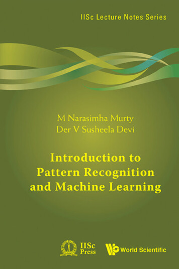
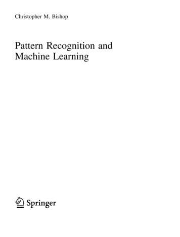
1IntroductionThe problem of searching for patterns in data is a fundamental one and has a long andsuccessful history. For instance, the extensive astronomical observations of TychoBrahe in the 16th century allowed Johannes Kepler to discover the empirical laws ofplanetary motion, which in turn provided a springboard for the development of classical mechanics. Similarly, the discovery of regularities in atomic spectra played akey role in the development and verification of quantum physics in the early twentieth century. The field of pattern recognition is concerned with the automatic discovery of regularities in data through the use of computer algorithms and with the use ofthese regularities to take actions such as classifying the data into different categories.Consider the example of recognizing handwritten digits, illustrated in Figure 1.1.Each digit corresponds to a 28 28 pixel image and so can be represented by a vectorx comprising 784 real numbers. The goal is to build a machine that will take such avector x as input and that will produce the identity of the digit 0, . . . , 9 as the output.This is a nontrivial problem due to the wide variability of handwriting. It could be1
21. INTRODUCTIONFigure 1.1Examples of hand-written digits taken from US zip codes.tackled using handcrafted rules or heuristics for distinguishing the digits based onthe shapes of the strokes, but in practice such an approach leads to a proliferation ofrules and of exceptions to the rules and so on, and invariably gives poor results.Far better results can be obtained by adopting a machine learning approach inwhich a large set of N digits {x1 , . . . , xN } called a training set is used to tune theparameters of an adaptive model. The categories of the digits in the training setare known in advance, typically by inspecting them individually and hand-labellingthem. We can express the category of a digit using target vector t, which representsthe identity of the corresponding digit. Suitable techniques for representing categories in terms of vectors will be discussed later. Note that there is one such targetvector t for each digit image x.The result of running the machine learning algorithm can be expressed as afunction y(x) which takes a new digit image x as input and that generates an outputvector y, encoded in the same way as the target vectors. The precise form of thefunction y(x) is determined during the training phase, also known as the learning
Pattern recognition has its origins in engineering, whereas machine learning grew out of computer science. However, these activities can be viewed as two facets of . that fill in important details, have solutions that are available as a PDF file from the book web site. Such