WIXLIB

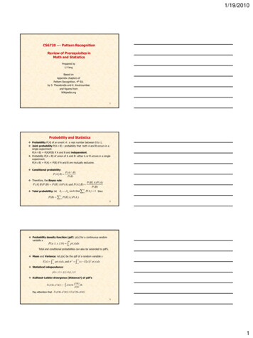
1/19/2010CS6720 --- Pattern RecognitionReview of Prerequisites inMath and StatisticsPrepared byLi YangBased onAppendix chapters ofPattern Recognition, 4th Ed.by S. Theodoridis and K. Koutroumbasand figures fromWikipedia.org1Probability and Statistics Probability P(A) of an event A : a real number between 0 to 1. Joint probability P(A B) : probability that both A and B occurs in asingle experiment.P(A B) P(A)P(B) if A and B and independent. Probability P(A B) of union of A and B: either A or B occurs in a singleexperiment.P(A B) P(A) P(B) if A and B are mutually exclusive. Conditional probability:P( A B) P( A B)P( B) Therefore, the Bayes rule:P( B A) P( A)P( B)m Total probability: let A1 ,., Am such that i 1 P( Ai ) 1 thenP ( A B ) P ( B) P ( B A) P ( A) and P( A B ) P( B) i 1 P( B Ai ) P( Ai )m2 Probability density function (pdf): p(x) for a continuous randomvariable xbP(a x b) p ( x)dxaTotal and conditional probabilities can also be extended to pdf’s. Mean and Variance: let p(x) be the pdf of a random variable x E[ x] xp ( x)dx, and 2 ( x E[ x])2 p( x)dx Statistical independence:p ( x, y ) p x ( x ) p y ( y ) Kullback-Leibler divergence (Distance?) of pdf’sL( p (x), p ' (x)) p (x) lnp ' ( x)dxp ( x)Pay attention that L( p(x), p' (x)) L( p' (x), p(x))31

1/19/2010 Characteristic function of a pdf: (Ω) p(x) exp( jΩT x)dx E[exp( jΩT x)] ( s ) p( x) exp( sx )dx E[exp(sx )] 2nd Characteristic function: (s) ln (s)d n (0) E[ x n ] n-th order moment:ds n Cumulants: d (0)nnndsWhen E[ x] 0, then 0 0, 1 E[ x] 0, 2 E[ x 2 ] 2 , 3 E[ x 3 ] (Skewness) 4 E[ x 4 ] 3 4 (Kurtosis)4Discrete Distributions Binomial distribution B(n,p):Repeatedly grab n balls, each with a probability p of getting a blackball. The probability of getting k black balls: n P(k ) p k (1 p) n k k Poisson distributionprobability of # of events occurring in a fixed period of time if theseevents occur with a known average.P(k ; ) k e k!When n and np remains constant,B(n, p) Poisson(np)5Normal (Gaussian) Distribution Univariate N(μ, σ2):p ( x) 1( x )2exp( )2 22 Multivariate N(μ, Σ):p( x) 1 1 exp ( x )T 1 ( x ) 2 2 with the mean and the covariance matrix 12 21 l1where i2 12 1l 22 2l l 2 l2 E[( xi i ) 2 ] and ij ji E[( xi i )( x j j )] Central limit theorem:Let z i 1 xi , thennz N (0,1) when n irrespective of the pdf' s of xi ' s.62

1/19/2010Other Continuous Distributions Chi-square (Χ2)distribution of k degrees of freedom:distribution of a sum of squares of k independent standard normalrandom variables, that is, 2 x12 x22 xk2 where xi N (0,1)p( y ) 1y k / 2 1e y / 2step( y ),2 k / 2 (k / 2) where ( z ) t z 1e t dt0 Mean: k, Variance: 2k2 Assume x (k ) Then( x k ) / 2k N (0,1) as k by central limit theorem. Also 2 x is approximately normally distributed with meanand unit variance.2k 17Other Continuous Distributions t-distribution: estimating mean of a normal distribution when samplesize is small.A t-distributed variable q x / z / k where x N (0,1) and z 2 (k )p(q) ((k 1) / 2) q 2 1 k k (k / 2) ( k 1) / 2Mean: 0 for k 1,variance: k/(k-2) for k 2 β-distribution: Beta(α,β): the posterior distribution of p of a binomialdistribution after α 1 events with p and β 1 with 1 p. ( ) 1x (1 x) 1 ( ) ( )1 x 1 (1 x) 1 ( , )p( x) 8Linear Algebra Eigenvalues and eigenvectors:there exists λ and v such that Av λv Real matrix A is called positive semidefinite if xTAx 0 for everynonzero vector x;A is called positive definite if xTAx 0. Positive definite matrixes act as positive numbers.All positive eigenvalues If A is symmetric, AT A,then its eigenvectors are orthogonal, viTvj 0. Therefore, a symmetric A can be diagonalized asA T and T A where [v1 , v2 , vl ] and diag ( 1 , 2 , l )93

1/19/2010Correlation Matrix and Inner Product MatrixPrincipal component analysis (PCA) Let x be a random variable in Rl, its correlation matrix Σ E[xxT] ispositive semidefinite and thus can be diagonalized as T Assign x' T x , then ' E ( x' x'T ) T Further assign x' ' 1/ 2 T x, then ' ' E ( x' ' x' 'T ) IClassical multidimensional scaling (classical MDS) Given a distance matrix D {dij}, the inner product matrix G {xiTxj} canbe computed by a bidirectional centering process111G ( I eeT ) D( I eeT ) where e [1,1,.,1]T2nn G can be diagnolized as G ' T Actually, nΛ and Λ’ share the same set of eigenvalues, and X T where X [ x1 ,.,xn ]TBecause G XX T , X can then be receovered as X '1/ 210Cost Function Optimization Find θ so that a differentiable function J(θ) is minimized. Gradient descent method Starts with an initial estimate θ(0) Adjust θ iteratively by new old J ( ) , where 0 old Taylor expansion of J(θ) at a stationary point θ01J ( ) J ( 0 ) ( 0 )T g ( 0 )T H( 0 ) O(( 0 )3 )2 J ( ) 2 J ( )where g 0 and H(i, j ) 0 i j Ignore higher order terms within a neighborhood of θ0 new 0 ( I H)( old 0 )H is positive semidefini te, then H T , we get T ( new 0 ) ( I ) T ( old 0 )which will converge if every 1 i 1, i.e., 2 / max.Therefore, the convergence speed is decided by min / max.11 Newton’s method Adjust θ iteratively by 1 H old J ( ) old Converges much faster that gradient descent.In fact, from the Taylor expansion, we have J ( ) H( 0 ) new old H 1 (H( old 0 )) 0 The minimum is found in one iteration. Conjugate gradient method t g t t t 1 J ( ) t g tT g tg T ( g g t 1 )and t Tor t t T tg t 1 g t 1g t 1 g t 1where g t 124

1/19/2010Constrained Optimization withEquality ConstraintsMinimize J(θ)subject to fi(θ) 0 for i 1, 2, , m Minimization happens at f ( ) J ( ) i Lagrange multipliers: constructmL( , ) J ( ) i f i ( )i 1and solve L( , ) L( , ) 0 13Constrained Optimization withInequality ConstraintsMinimize J(θ) subject to fi(θ) 0 for i 1, 2, , m fi(θ) 0 i 1, 2, , m defines a feasible region in which the answer lies. Karush–Kuhn–Tucker (KKT) conditions:A set of necessary conditions, which a local optimizer θ* has to satisfy.There exists a vector λ of Lagrange multipliers such that (1)L(θ* , λ ) 0 θ(2) i 0 for i 1,2,.,m(3) i f i (θ* ) 0 for i 1,2,.,m(1) Most natural condition.(2) fi(θ*) is inactive if λi 0.(3) λi 0 if the minimum is on fi(θ*).(4) The (unconstrained) minimum in the interior region if all λi 0.(5) For convex J(θ) and the region, local minimum is global minimum.(6) Still difficult to compute. Assume some fi(θ*)’s active, check λi 0.14 Convex function:f ( ) :S l is convax if θ,θ' S , [0,1]f ( (1 ) ' ) f ( ) (1 ) f ( ' ) Concave function:f ( (1 ) ' ) f ( ) (1 ) f ( ' ) Convex set:S l is a convax set if θ,θ' S , [0,1] (1 ) ' ) SLocal minimum of a convex function is also global minimum.If f ( ) is concave, then X { f ( ) b} is a convex set.155

1/19/2010 Min-Max dualityGame : A pays F ( x, y ) to B while A chooses x and B chooses yA' s goal : min max F ( x, y ), B' s goal : max min F ( x, y )xyxyThe two problems are dual to each other.In general : min F ( x, y ) F ( x, y ) max F ( x, y )xyTherefore, max min F ( x, y ) min max F ( x, y )xyxySaddle point condition :If there exists ( x* ,y* ) such thatF ( x* , y ) F ( x* , y* ) F ( x, y* )or equivalent ly :F ( x* , y* ) max min F ( x, y ) min max F ( x, y )xyxy16 Lagrange duality Recall the optimization problem:Minimize J ( )s.t. f i ( ) 0 for i 1,2,.,mmLagrange function : L( , ) J ( ) i f i ( )i 1Because max L( , ) J ( ), we have 0min J ( ) min max L( , ) 0 Convex ProgrammingFor a large class of applicatio ns, J ( ) is convex, f i ( )' s are concavethen, the minimizati on solution ( * , * ) is a saddle point of L( , )L( * , ) L( * , * ) L( , * )L( * , * ) min max L( , ) max min L( , ) 0 0 Therefore, the optimizati on problem becomes max min L( , ), or 0max L( , ) 0subject to L( , ) 0 MUCH SIMPLER!17Mercer’s Theorem and the Kernel Method Mercer’s theorem:Let x l and given a mapping ( x) H ,( H denotes Hilbert space, i.e. finite or infinite Euclidean space)the inner product ( x), ( y ) can be expressed as a kernelfunction ( x), ( y ) K ( x, y )where K ( x, y ) is symmetric, continuous, and positive semi - definite.The opposite is also true.The kernel method can transform any algorithm that solely depends onthe dot product between two vectors to a kernelized vesion, byreplacing dot product with the kernel function. The kernelized versionis equivalent to the algorithm operating in the range space of φ.Because kernels are used, however, φ is never explicitly computed.186

CS6720 --- Pattern Recognition Review of Prerequisites in Math and Statistics Prepared by Li Yang Based on Appendix chapters of Pattern Recognition, 4th Ed. by S. Theodoridis and K. Koutroumbas and figures from Wikipedia.org 1 Probability and Statistics Prob